Any logical expression can be used as an index which opens a wide
range of possibilities. For example, you can remove or focus on
entries that match specific criteria. For example, you might want to
remove all entries that are above a certain value:
For another example, suppose you want to join together the values that
match two different factors in another vector:
Note that a single ‘|’ was used in the previous example. There is a
difference between ‘||’ and ‘|’. A single bar will perform a vector
operation, term by term, while a double bar will evaluate to a single
TRUE or FALSE result:
Here we look at the most basic linear least squares regression. The
main purpose is to provide an example of the basic commands. It is
assumed that you know how to enter data or read data files which is
covered in the first chapter, and it is assumed that you are familiar
with the different data types.
We will examine the interest rate for four year car loans, and the
data that we use comes from the
U.S. Federal Reserve’s mean rates .
We are looking at and plotting means. This, of course, is a very bad
thing because it removes a lot of the variance and is misleading. The
only reason that we are working with the data in this way is to
provide an example of linear regression that does not use too many
data points. Do not try this without a professional near you, and if a
professional is not near you do not tell anybody you did this. They
will laugh at you. People are mean, especially professionals.
The first thing to do is to specify the data. Here there are only five
pairs of numbers so we can enter them in manually. Each of the five
pairs consists of a year and the mean interest rate:
The next thing we do is take a look at the data. We first plot the
data using a scatter plot and notice that it looks linear. To confirm
our suspicions we then find the correlation between the year and the
mean interest rates:
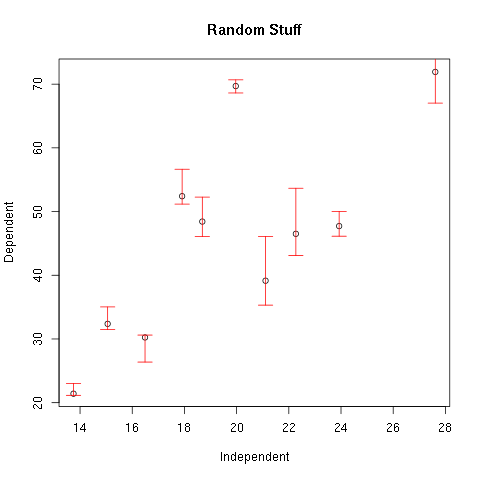
> plot(year,rate,
main="Commercial Banks Interest Rate for 4 Year Car Loan",
sub="http://www.federalreserve.gov/releases/g19/20050805/")
> cor(year,rate)
[1] -0.9880813
exercise:
year <- c(2000 , 2001 , 2002 , 2003 , 2004)
rate <- c(9.34 , 8.50 , 7.62 , 6.93 , 6.60)
plot(year,rate,
main="Commercial Banks Interest Rate for 4 Year Car Loan",
sub="http://www.federalreserve.gov/releases/g19/20050805/")
cor(year,rate)
fit <- lm(rate ~ year)
fit
attributes(fit)
names(fit)
length(fit)
fit$coefficients[[2]]*2015+fit$coefficients[[1]]
At this point we should be excited because associations that strong
never happen in the real world unless you cook the books or work with
averaged data. The next question is what straight line comes “closest”
to the data? In this case we will use least squares regression as one
way to determine the line.
Before we can find the least square regression line we have to make
some decisions. First we have to decide which is the explanatory and
which is the response variable. Here, we arbitrarily pick the
explanatory variable to be the year, and the response variable is the
interest rate. This was chosen because it seems like the interest rate
might change in time rather than time changing as the interest rate
changes. (We could be wrong, finance is very confusing.)
The command to perform the least square regression is the lm
command. The command has many options, but we will keep it simple and
not explore them here. If you are interested use the help(lm) command
to learn more. Instead the only option we examine is the one necessary
argument which specifies the relationship.
Since we specified that the interest rate is the response variable and
the year is the explanatory variable this means that the regression
line can be written in slope-intercept form:
\[rate = (slope) year + (intercept)\]
The way that this relationship is defined in the lm command is that
you write the vector containing the response variable, a tilde (“~”),
and a vector containing the explanatory variable:
> fit <- lm(rate ~ year)
> fit
Call:
lm(formula = rate ~ year)
Coefficients:
(Intercept) year
1419.208 -0.705
When you make the call to lm it returns a variable with a lot of
information in it. If you are just learning about least squares
regression you are probably only interested in two things at this
point, the slope and the y-intercept. If you just type the name of the
variable returned by lm it will print out this minimal information to
the screen. (See above.)
If you would like to know what else is stored in the variable you can
use the attributes command:
> attributes(fit)
$names
[1] "coefficients" "residuals" "effects" "rank"
[5] "fitted.values" "assign" "qr" "df.residual"
[9] "xlevels" "call" "terms" "model"
$class
[1] "lm"
One of the things you should notice is the coefficients variable
within fit. You can print out the y-intercept and slope by accessing
this part of the variable:
> fit$coefficients[1]
(Intercept)
1419.208
> fit$coefficients[[1]]
[1] 1419.208
> fit$coefficients[2]
year
-0.705
> fit$coefficients[[2]]
[1] -0.705
Note that if you just want to get the number you should use two square
braces. So if you want to get an estimate of the interest rate in the
year 2015 you can use the formula for a line:
> fit$coefficients[[2]]*2015+fit$coefficients[[1]]
[1] -1.367
So if you just wait long enough, the banks will pay you to take a car!
A better use for this formula would be to calculate the residuals and
plot them:
> res <- rate - (fit$coefficients[[2]]*year+fit$coefficients[[1]])
> res
[1] 0.132 -0.003 -0.178 -0.163 0.212
> plot(year,res)
That is a bit messy, but fortunately there are easier ways to get the
residuals. Two other ways are shown below:
> residuals(fit)
1 2 3 4 5
0.132 -0.003 -0.178 -0.163 0.212
> fit$residuals
1 2 3 4 5
0.132 -0.003 -0.178 -0.163 0.212
> plot(year,fit$residuals)
>
If you want to plot the regression line on the same plot as your
scatter plot you can use the abline function along with your variable
fit:
> plot(year,rate,
main="Commercial Banks Interest Rate for 4 Year Car Loan",
sub="http://www.federalreserve.gov/releases/g19/20050805/&quo, .toc-backreft;)
> abline(fit)
Finally, as a teaser for the kinds of analyses you might see later,
you can get the results of an F-test by asking R for a summary of the
fit variable:
> summary(fit)
Call:
lm(formula = rate ~ year)
Residuals:
1 2 3 4 5
0.132 -0.003 -0.178 -0.163 0.212
Coefficients:
Estimate Std. Error t value Pr(>|t|)
(Intercept) 1419.20800 126.94957 11.18 0.00153 **
year -0.70500 0.06341 -11.12 0.00156 **
---
Signif. codes: 0 '***' 0.001 '**' 0.01 '*' 0.05 '.' 0.1 ' ' 1
Residual standard error: 0.2005 on 3 degrees of freedom
Multiple R-Squared: 0.9763, Adjusted R-squared: 0.9684
F-statistic: 123.6 on 1 and 3 DF, p-value: 0.001559
9. Calculating Confidence Intervals
Here we look at some examples of calculating confidence intervals. The
examples are for both normal and t distributions. We assume that you
can enter data and know the commands associated with basic
probability. Note that an easier way to calculate confidence intervals
using the t.test command is discussed in section The Easy Way.
Here we will look at a fictitious example. We will make some
assumptions for what we might find in an experiment and find the
resulting confidence interval using a normal distribution. Here we
assume that the sample mean is 5, the standard deviation is 2, and the
sample size is 20. In the example below we will use a 95% confidence
level and wish to find the confidence interval. The commands to find
the confidence interval in R are the following:
> a <- 5
> s <- 2
> n <- 20
> error <- qnorm(0.975)*s/sqrt(n)
> left <- a-error
> right <- a+error
> left
[1] 4.123477
> right
[1] 5.876523
Our level of certainty about the true mean is 95% in predicting that the
true mean is within the interval
between 4.12 and 5.88 assuming that the original random variable is
normally distributed, and the samples are independent.
Calculating the confidence interval when using a t-test is similar to
using a normal distribution. The only difference is that we use the
command associated with the t-distribution rather than the normal
distribution. Here we repeat the procedures above, but we will assume
that we are working with a sample standard deviation rather than an
exact standard deviation.
Again we assume that the sample mean is 5, the sample standard
deviation is 2, and the sample size is 20. We use a 95% confidence
level and wish to find the confidence interval. The commands to find
the confidence interval in R are the following:
> a <- 5
> s <- 2
> n <- 20
> error <- qt(0.975,df=n-1)*s/sqrt(n)
> left <- a-error
> right <- a+error
> left
[1] 4.063971
> right
[1] 5.936029
The true mean has a probability of 95% of being in the interval
between 4.06 and 5.94 assuming that the original random variable is
normally distributed, and the samples are independent.
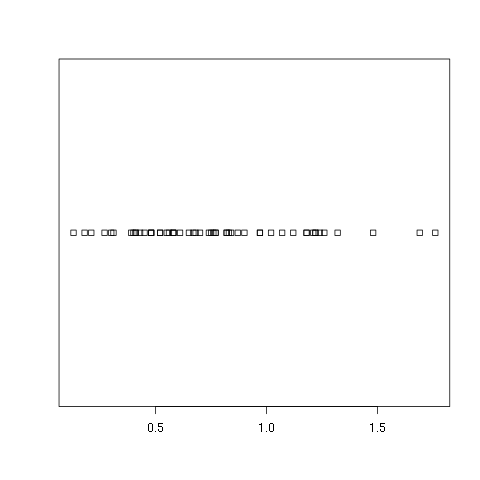
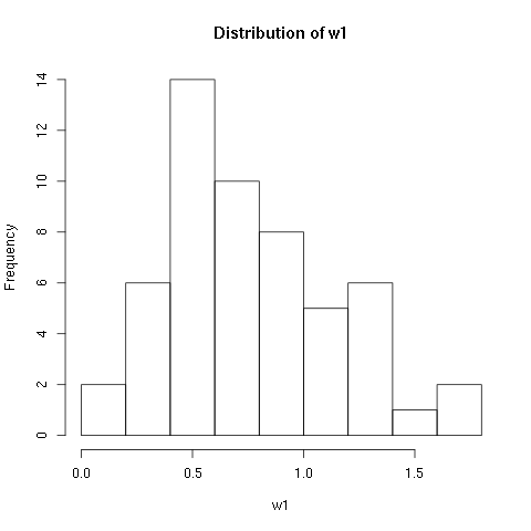
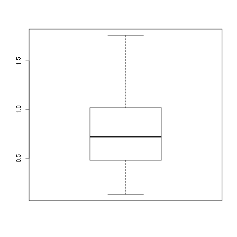
We now look at an example where we have a univariate data set and want
to find the 95% confidence interval for the mean. In this example we
use one of the data sets given in the data input chapter. We use the
w1.dat data set:
> w1 <- read.csv(file="w1.dat",sep=",",head=TRUE)
, .toc-backref> summary(w1)
vals
Min. :0.130
1st Qu.:0.480
Median :0.720
Mean :0.765
3rd Qu.:1.008
Max. :1.760
> length(w1$vals)
[1] 54
> mean(w1$vals)
[1] 0.765
> sd(w1$vals)
[1] 0.3781222
We can now calculate an error for the mean:
> error <- qt(0.975,df=length(w1$vals)-1)*sd(w1$vals)/sqrt(length(w1$vals))
> error
[1] 0.1032075
The confidence interval is found by adding and subtracting the error
from the mean:
> left <- mean(w1$vals)-error
> right <- mean(w1$vals)+error
> left
[1] 0.6617925
> right
[1] 0.8682075
There is a 95% probability that the true mean is between 0.66 and 0.87
assuming that the original random variable is normally distributed,
and the samples are independent.
Suppose that you want to find the confidence intervals for many
tests. This is a common task and most software packages will allow you
to do this.
We have three different sets of results:
| Comparison 1 |
|
|
| |
Mean |
Std. Dev. |
Number (pop.) |
| Group I |
10 |
3 |
300 |
| Group II |
10.5 |
2.5 |
230 |
| Comparison 2 |
|
|
| |
Mean |
Std. Dev. |
Number (pop.) |
| Group I |
12 |
4 |
210 |
| Group II |
13 |
5.3 |
340 |
| Comparison 3 |
|
|
| |
Mean |
Std. Dev. |
Number (pop.) |
| Group I |
30 |
4.5 |
420 |
| Group II |
28.5 |
3 |
400 |
For each of these comparisons we want to calculate the associated
confidence interval for the difference of the means. For each
comparison there are two groups. We will refer to group one as the
group whose results are in the first row of each comparison above. We
will refer to group two as the group whose results are in the second
row of each comparison above. Before we can do that we must first
compute a standard error and a t-score. We will find general formulae
which is necessary in order to do all three calculations at once.
We assume that the means for the first group are defined in a variable
called m1. The means for the second group are defined in a variable
called m2. The standard deviations for the first group are in a
variable called sd1. The standard deviations for the second group
are in a variable called sd2. The number of samples for the first
group are in a variable called num1. Finally, the number of samples
for the second group are in a variable called num2.
With these definitions the standard error is the square root of
(sd1^2)/num1+(sd2^2)/num2. The R commands to do this can be found
below:
> m1 <- c(10,12,30)
> m2 <- c(10.5,13,28.5)
> sd1 <- c(3,4,4.5)
> sd2 <- c(2.5,5.3,3)
> num1 <- c(300,210,420)
> num2 <- c(230,340,400)
> se <- sqrt(sd1*sd1/num1+sd2*sd2/num2)
> error <- qt(0.975,df=pmin(num1,num2)-1)*se
To see the values just type in the variable name on a line alone:
> m1
[1] 10 12 30
> m2
[1] 10.5 13.0 28.5
> sd1
[1] 3.0 4.0 4.5
> sd2
[1] 2.5 5.3 3.0
> num1
[1] 300 210 420
> num2
[1] 230 340 400
> se
[1] 0.2391107 0.3985074 0.2659216
> error
[1] 0.4711382 0.7856092 0.5227825
Now we need to define the confidence interval around the assumed
differences. Just as in the case of finding the p values in previous
chapter we have to use the pmin command to get the number of degrees
of freedom. In this case the null hypotheses are for a difference of
zero, and we use a 95% confidence interval:
> left <- (m1-m2)-error
> right <- (m1-m2)+error
> left
[1] -0.9711382 -1.7856092 0.9772175
> right
[1] -0.02886177 -0.21439076 2.02278249
This gives the confidence intervals for each of the three tests. For
example, in the first experiment the 95% confidence interval is
between -0.97 and -0.03 assuming that the random variables are
normally distributed, and the samples are independent.
10. Calculating p Values
Here we look at some examples of calculating p values. The examples
are for both normal and t distributions. We assume that you can enter
data and know the commands associated with basic probability. We first
show how to do the calculations the hard way and show how to do the
calculations. The last method makes use of the t.test command and
demonstrates an easier way to calculate a p value.
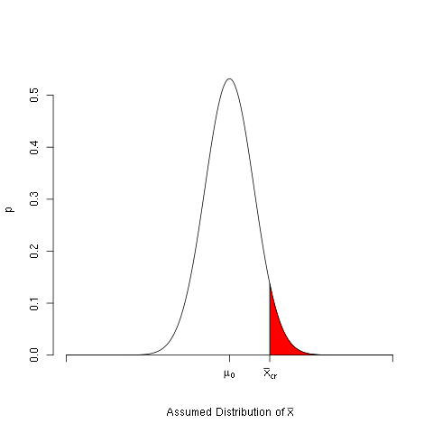
We look at the steps necessary to calculate the p value for a
particular test. In the interest of simplicity we only look at a two
sided test, and we focus on one example. Here we want to show that the
mean is not close to a fixed value, a.
\[\begin{split}H_o: \mu_x & = & a,\end{split}\]\[\begin{split}H_a: \mu_x & \neq & a,\end{split}\]
The p value is calculated for a particular sample mean. Here we assume
that we obtained a sample mean, x and want to find its p value. It is
the probability that we would obtain a given sample mean that is
greater than the absolute value of its Z-score or less than the
negative of the absolute value of its Z-score.
For the special case of a normal distribution we also need the
standard deviation. We will assume that we are given the standard
deviation and call it s. The calculation for the p value can be done
in several of ways. We will look at two ways here. The first way is to
convert the sample means to their associated Z-score. The other way is
to simply specify the standard deviation and let the computer do the
conversion. At first glance it may seem like a no brainer, and we
should just use the second method. Unfortunately, when using the
t-distribution we need to convert to the t-score, so it is a good idea
to know both ways.
We first look at how to calculate the p value using the Z-score. The
Z-score is found by assuming that the null hypothesis is true,
subtracting the assumed mean, and dividing by the theoretical standard
deviation. Once t, .toc-backrefhe Z-score is found the probability that the value
could be less the Z-score is found using the pnorm command.
This is not enough to get the p value. If the Z-score that is found is
positive then we need to take one minus the associated
probability. Also, for a two sided test we need to multiply the result
by two. Here we avoid these issues and insure that the Z-score is
negative by taking the negative of the absolute value.
We now look at a specific example. In the example below we will use a
value of a of 5, a standard deviation of 2, and a sample size
of 20. We then find the p value for a sample mean of 7:
> a <- 5
> s <- 2
> n <- 20
> xbar <- 7
> z <- (xbar-a)/(s/sqrt(n))
> z
[1] 4.472136
> 2*pnorm(-abs(z))
[1] 7.744216e-06
We now look at the same problem only specifying the mean and standard
deviation within the pnorm command. Note that for this case we cannot
so easily force the use of the left tail. Since the sample mean is
more than the assumed mean we have to take two times one minus the
probability:
> a <- 5
> s <- 2
> n <- 20
> xbar <- 7
> 2*(1-pnorm(xbar,mean=a,sd=s/sqrt(20)))
[1] 7.744216e-06
Finding the p value using a t distribution is very similar to using
the Z-score as demonstrated above. The only difference is that you
have to specify the number of degrees of freedom. Here we look at the
same example as above but use the t distribution instead:
> a <- 5
> s <- 2
> n <- 20
> xbar <- 7
> t <- (xbar-a)/(s/sqrt(n))
> t
[1] 4.472136
> 2*pt(-abs(t),df=n-1)
[1] 0.0002611934
We now look at an example where we have a univariate data set and want
to find the p value. In this example we use one of the data sets given
in the data input chapter. We use the w1.dat data set:
> w1 <- read.csv(file="w1.dat",sep=",",head=TRUE)
> summary(w1)
vals
Min. :0.130
1st Qu.:0.480
Median :0.720
Mean :0.765
3rd Qu.:1.008
Max. :1.760
> length(w1$vals)
[1] 54
Here we use a two sided hypothesis test,
\[\begin{split}H_o: \mu_x & = & 0.7,\end{split}\]\[\begin{split}H_a: \mu_x & \neq & 0.7.\end{split}\]
So we calculate the sample mean and sample standard deviation in order
to calculate the p value:
> t <- (mean(w1$vals)-0.7)/(sd(w1$vals)/sqrt(length(w1$vals)))
> t
[1] 1.263217
> 2*pt(-abs(t),df=length(w1$vals)-1)
[1] 0.21204
Suppose that you want to find the p values for many tests. This is a
common task and most software packages will allow you to do this. Here
we see how it can be done in R.
Here we assume that we want to do a one-sided hypothesis test for a
number of comparisons. In particular we will look at three hypothesis
tests. All are of the following form:
\[\begin{split}H_o: \mu_1 - \mu_2 & = & 0,\end{split}\]\[\begin{split}H_a: \mu_1 - \mu_2 & \neq & 0.\end{split}\]
We have three different sets of comparisons to make:
| Comparison |
1 |
|
|
| |
Mean |
Std. Dev. |
Number
(pop.) |
| Group I |
10 |
3 |
300 |
| Group II |
10.5 |
2.5 |
230 |
| Comparison |
2 |
|
|
| |
Mean |
Std. Dev. |
Number
(pop.) |
| Group I |
12 |
4 |
210 |
| Group II |
13 |
5.3 |
340 |
| Comparison |
3 |
|
|
| |
Mean |
Std. Dev. |
Number
(pop.) |
| Group I |
30 |
4.5 |
420 |
| Group II |
28.5 |
3 |
400 |
For each of these comparisons we want to calculate a p value. For each
comparison there are two groups. We will refer to group one as the
group whose results are in the first row of each comparison above. We
will refer to group two as the group whose results are in the second
row of each comparison above. Before we can do that we must first
compute a standard error and a t-score. We will find general formulae
which is necessary in order to do all three calculations at once.
We assume that the means for the first group are defined in a variable
called m1. The means for the second group are defined in a variable
called m2. The standard deviations for the first group are in a
variable called sd1. The standard deviations for the second group are
in a variable called sd2. The number of samples for the first group
are in a variable called num1. Finally, the number of samples for the
second group are in a variable called num2.
With these definitions the standard error is the square root of
(sd1^2)/num1+(sd2^2)/num2. The associated t-score is m1 minus m2
all divided by the standard error. The R comands to do this can be
found below:
> m1 <- c(10,12,30)
> m2 <- c(10.5,13,28.5)
> sd1 <- c(3,4,4.5)
> sd2 <- c(2.5,5.3,3)
> num1 <- c(300,210,420)
> num2 <- c(230,340,400)
> se <- sqrt(sd1*sd1/num1+sd2*sd2/num2)
> t <- (m1-m2)/se
To see the values just type in the vari, .toc-backrefable name on a line alone:
> m1
[1] 10 12 30
> m2
[1] 10.5 13.0 28.5
> sd1
[1] 3.0 4.0 4.5
> sd2
[1] 2.5 5.3 3.0
> num1
[1] 300 210 420
> num2
[1] 230 340 400
> se
[1] 0.2391107 0.3985074 0.2659216
> t
[1] -2.091082 -2.509364 5.640761
To use the pt command we need to specify the number of degrees of
freedom. This can be done using the pmin command. Note that there is
also a command called min, but it does not work the same way. You
need to use pmin to get the correct results. The numbers of degrees
of freedom are pmin(num1,num2)-1. So the p values can be found
using the following R command:
> pt(t,df=pmin(num1,num2)-1)
[1] 0.01881168 0.00642689 0.99999998
If you enter all of these commands into R you should have noticed that
the last p value is not correct. The pt command gives the probability
that a score is less that the specified t. The t-score for the last
entry is positive, and we want the probability that a t-score is
bigger. One way around this is to make sure that all of the t-scores
are negative. You can do this by taking the negative of the absolute
value of the t-scores:
> pt(-abs(t),df=pmin(num1,num2)-1)
[1] 1.881168e-02 6.426890e-03 1.605968e-08
The results from the command above should give you the p values for a
one-sided test. It is left as an exercise how to find the p values for
a two-sided test.
The methods above demonstrate how to calculate the p values directly
making use of the standard formulae. There is another, more direct way
to do this using the t.test command. The t.test command takes a
data set for an argument, and the default operation is to perform a
two sided hypothesis test.
> x = c(9.0,9.5,9.6,10.2,11.6)
> t.test(x)
One Sample t-test
data: x
t = 22.2937, df = 4, p-value = 2.397e-05
alternative hypothesis: true mean is not equal to 0
95 percent confidence interval:
8.737095 11.222905
sample estimates:
mean of x
9.98
> help(t.test)
>
That was an obvious result. If you want to test against a
different assumed mean then you can use the mu argument:
> x = c(9.0,9.5,9.6,10.2,11.6)
> t.test(x,mu=10)
One Sample t-test
data: x
t = -0.0447, df = 4, p-value = 0.9665
alternative hypothesis: true mean is not equal to 10
95 percent confidence interval:
8.737095 11.222905
sample estimates:
mean of x
9.98
If you are interested in a one sided test then you can specify which
test to employ using the alternative option:
> x = c(9.0,9.5,9.6,10.2,11.6)
> t.test(x,mu=10,alternative="less")
One Sample t-test
data: x
t = -0.0447, df = 4, p-value = 0.4833
alternative hypothesis: true mean is less than 10
95 percent confidence interval:
-Inf 10.93434
sample estimates:
mean of x
9.98
The t.test, .toc-backref() command also accepts a second data set to compare two
sets of samples. The default is to treat them as independent sets, but
there is an option to treat them as dependent data sets. (Enter
help(t.test) for more information.) To test two different samples,
the first two arguments should be the data sets to compare:
> x = c(9.0,9.5,9.6,10.2,11.6)
> y=c(9.9,8.7,9.8,10.5,8.9,8.3,9.8,9.0)
> t.test(x,y)
Welch Two Sample t-test
data: x and y
t = 1.1891, df = 6.78, p-value = 0.2744
alternative hypothesis true difference in means is not equal to 0
95 percent confidence interval:
-0.6185513 1.8535513
sample estimates:
mean of x mean of y
9.9800 9.3625
11. Calculating The Power Of A Test
Here we look at some examples of calculating the power of a test. The
examples are for both normal and t distributions. We assume that you
can enter data and know the commands associated with basic
probability. All of the examples here are for a two sided test, and
you can adjust them accordingly for a one sided test.
Here we calculate the power of a test for a normal distribution for a
specific example. Suppose that our hypothesis test is the following:
\[\begin{split}H_o: \mu_x & = & a,\end{split}\]\[\begin{split}H_a: \mu_x & \neq & a,\end{split}\]
The power of a test is the probability that we can the reject null
hypothesis at a given mean that is away from the one specified in the
null hypothesis. We calculate this probability by first calculating
the probability that we accept the null hypothesis when we should
not. This is the probability to make a type II error. The power is the
probability that we do not make a type II error so we then take one
minus the result to get the power.
We can fail to reject the null hypothesis if the sample happens to be
within the confidence interval we find when we assume that the null
hypothesis is true. To get the confidence interval we find the margin
of error and then add and subtract it to the proposed mean, a, to get
the confidence interval. We then turn around and assume instead that
the true mean is at a different, explicitly specified level, and then
find the probability a sample could be found within the original
confidence interval.
In the example below the hypothesis test is for
\[\begin{split}H_o: \mu_x & = & 5,\end{split}\]\[\begin{split}H_a: \mu_x & \neq & 5,\end{split}\]
We will assume that the standard deviation is 2, and the sample size
is 20. In the example below we will use a 95% confidence level and
wish to find the power to detect a true mean that differs from 5 by an
amount of 1.5. (A, .toc-backrefll of these numbers are made up solely for this
example.) The commands to find the confidence interval in R are the
following:
> a <- 5
> s <- 2
> n <- 20
> error <- qnorm(0.975)*s/sqrt(n)
> left <- a-error
> right <- a+error
> left
[1] 4.123477
> right
[1] 5.876523
Next we find the Z-scores for the left and right values assuming that the true mean is 5+1.5=6.5:
> assumed <- a + 1.5
> Zleft <- (left-assumed)/(s/sqrt(n))
> Zright <-(right-assumed)/(s/sqrt(n))
> p <- pnorm(Zright)-pnorm(Zleft)
> p
[1] 0.08163792
The probability that we make a type II error if the true mean is 6.5
is approximately 8.1%. So the power of the test is 1-p:
In this example, the power of the test is approximately 91.8%. If the
true mean differs from 5 by 1.5 then the probability that we will
reject the null hypothesis is approximately 91.8%.
Calculating the power when using a t-test is similar to using a normal
distribution. One difference is that we use the command associated
with the t-distribution rather than the normal distribution. Here we
repeat the test above, but we will assume that we are working with a
sample standard deviation rather than an exact standard deviation. We
will explore three different ways to calculate the power of a
test. The first method makes use of the scheme many books recommend if
you do not have the non-central distribution available. The second
does make use of the non-central distribution, and the third makes use
of a single command that will do a lot of the work for us.
In the example the hypothesis test is the same as above,
\[\begin{split}H_o: \mu_x & = & 5,\end{split}\]\[\begin{split}H_a: \mu_x & \neq & 5,\end{split}\]
Again we assume that the sample standard deviation is 2, and the
sample size is 20. We use a 95% confidence level and wish to find the
power to detect a true mean that differs from 5 by an amount of
1.5. The commands to find the confidence interval in R are the
following:
> a <- 5
> s <- 2
> n <- 20
> error <- qt(0.975,df=n-1)*s/sqrt(n)
> left <- a-error
> right <- a+error
> left
[1] 4.063971
> right
[1] 5.936029
The number of observations is large enough that the results are quite
close to those in the example using the normal distribution. Next we
find the t-scores for the left and right values assuming that the true
mean is 5+1.5=6.5:
> assumed <- a + 1.5
> tleft <- (left-assumed)/(s/sqrt(n))
> tright <- (right-assumed)/(s/sqrt(n))
> p <- pt(tright,df=n-1)-pt(tleft,df=n-1)
> p
[1] 0.1112583
The probability that we make a type II error if the true mean is 6.5
is approximately 11.1%. So the power of the test is 1-p:
In this example, the power of the test is approximately 88.9%. If the
true mean differs from 5 by 1.5 then the probability that we will
reject the null hypothesis is approximately 88.9%. Note that the power
calculated for a normal distribution is slightly higher than for this
one calculated with the t-distribution.
Another way to approximate the power is to make use of the
non-centrality parameter. The idea is that you give it the critical t
scores and the amount that the mean would be shifted if the alternate
mean were the true mean. This is the method that most books recommend.
> ncp <- 1.5/, .toc-backref(s/sqrt(n))
> t <- qt(0.975,df=n-1)
> pt(t,df=n-1,ncp=ncp)-pt(-t,df=n-1,ncp=ncp)
[1] 0.1111522
> 1-(pt(t,df=n-1,ncp=ncp)-pt(-t,df=n-1,ncp=ncp))
[1] 0.8888478
Again, we see that the probability of making a type II error is
approximately 11.1%, and the power is approximately 88.9%. Note that
this is slightly different than the previous calculation but is still
close.
Finally, there is one more command that we explore. This command
allows us to do the same power calculation as above but with a single
command.
> power.t.test(n=n,delta=1.5,sd=s,sig.level=0.05,
type="one.sample",alternative="two.sided",strict = TRUE)
One-sample t test power calculation
n = 20
delta = 1.5
sd = 2
sig.level = 0.05
power = 0.8888478
alternative = two.sided
This is a powerful command that can do much more than just calculate
the power of a test. For example it can also be used to calculate the
number of observations necessary to achieve a given power. For more
information check out the help page, help(power.t.test).
Suppose that you want to find the powers for many tests. This is a
common task and most software packages will allow you to do this. Here
we see how it can be done in R. We use the exact same cases as in the
previous chapter.
Here we assume that we want to do a two-sided hypothesis test for a
number of comparisons and want to find the power of the tests to
detect a 1 point difference in the means. In particular we will look
at three hypothesis tests. All are of the following form:
\[\begin{split}H_o: \mu_1 - \mu2 & = & 0,\end{split}\]\[\begin{split}H_a: \mu_1 - \mu_2 & \neq & 0,\end{split}\]
We have three different sets of comparisons to make:
| Comparison 1 |
|
|
| |
Mean |
Std. Dev. |
Number
(pop.) |
| Group I |
10 |
3 |
300 |
| Group II |
10.5 |
2.5 |
230 |
| Comparison 2 |
|
|
| |
Mean |
Std.
Dev. |
Number
(pop.) |
| Group I |
12 |
4 |
210 |
| Group II |
13 |
5.3 |
340 |
| Comparison 3 |
|
|
| |
Mean |
Std.
Dev. |
Number
(pop.) |
| Group I |
30 |
4.5 |
420 |
| Group II |
28.5 |
3 |
400 |
For each of these comparisons we want to calculate the power of the
test. For each comparison there are two groups. We will refer to group
one as the group whose results are in the first row of each comparison
above. We will refer to group two as the group whose results are in
the second row of each comparison above. Before we can do that we must
first compute a standard error and a t-score. We will find general
formulae which is necessary in order to do all three calculations at
once.
We assume that the means for the first group are defined in a variable
called m1. The means for the second group are defined in a variable
called m2. The standard deviations for the first group are in a
variable called sd1. The standard deviations for the second group are
in a variable called sd2. The number of samples for the first group
are in a variable called num1. Finally, the number of samples for the
second group are in a variable called num2.
With these definitions the standard error is the square root of
(sd1^2)/num1+(sd2^2)/num2. The R commands to do this can be found
below:
> m1 <- c(10,12,30)
> m2 <- c(10.5,13,28.5)
> sd1 <- c(3,4,4.5)
> sd2 <- c(2.5,5.3,3)
> num1 <- c(300,210,420)
> num2 <- c(230,340,400)
> se <- sqrt(sd1*sd1/num1+sd2*sd2/num2)
To see the values just type in the variable name on a line alone:
> m1
[1] 10 12 30
> m2
[1] 10.5 13.0 28.5
> sd1
[1] 3.0 4.0 4.5
> sd2
[1] 2.5 5.3 3.0
> num1
[1] 300 210 420
> num2
[1] 230 340 400
> se
[1] 0.2391107 0.3985074 0.2659216
Now we need to define the confidence interval around the assumed
differences. Just as in the case of finding the p values in previous
chapter we have to use the pmin command to get the number of degrees
of freedom. In this case the null hypotheses are for a difference of
zero, and we use a 95% confidence interval:
> left <- qt(0.025,df=pmin(num1,num2)-1)*se
> right <- -left
> left
[1] -0.4711382 -0.7856092 -0.5227825
> right
[1] 0.4711382 0.7856092 0.5227825
We can now calculate the power of the one sided test. Assuming a true
mean of 1 we can calculate the t-scores associated with both the left
and right variables:
> tl <- (left-1)/se
> tr <- (right-1)/se
> tl
[1] -6.152541 -4.480743 -5.726434
> tr
[1] -2.2117865 -0.5379844 -1.7945799
> probII <- pt(tr,df=pmin(num1,num2)-1) -
pt(tl,df=pmin(num1,num2)-1)
> probII
[1] 0.01398479 0.29557399 0.03673874
> power <- 1-probII
> power
[1] 0.9860152 0.7044260 0.9632613
The results from the command above should give you the p-values for a
two-sided test. It is left as an exercise how to find the p-values for
a one-sided test.
Just as was found above there is more than one way to calculate the
power. We also include the method using the non-central parameter
which is recommen, .toc-backrefded over the previous method:
> t <- qt(0.975,df=pmin(num1,num2)-1)
> t
[1] 1.970377 1.971379 1.965927
> ncp <- (1)/se
> pt(t,df=pmin(num1,num2)-1,ncp=ncp)-pt(-t,df=pmin(num1,num2)-1,ncp=ncp)
[1] 0.01374112 0.29533455 0.03660842
> 1-(pt(t,df=pmin(num1,num2)-1,ncp=ncp)-pt(-t,df=pmin(num1,num2)-1,ncp=ncp))
[1] 0.9862589 0.7046655 0.9633916
12. Two Way Tables
Here we look at some examples of how t, .toc-backrefo work with two way tables. We
assume that you can enter data and understand the different data
types.
We first look at how to create a table from raw data. Here we use a
fictitious data set, smoker.csv. This data set
was created only to be used as an example, and the numbers were
created to match an example from a text book, p. 629 of the 4th
edition of Moore and McCabe’s Introduction to the Practice of
Statistics. You should look at the data set in a spreadsheet to see
how it is entered. The information is ordered in a way to make it
easier to figure out what information is in the data.
The idea is that 356 people have been polled on their smoking status
(Smoke) and their socioeconomic status (SES). For each person it was
determined whether or not they are current smokers, former smokers, or
have never smoked. Also, for each person their socioeconomic status
was determined (low, middle, or high). The data file contains only two
columns, and when read R interprets them both as factors:
> smokerData <- read.csv(file='smoker.csv',sep=',',header=T)
> summary(smokerData)
Smoke SES
current:116 High :211
former :141 Low : 93
never : 99 Middle: 52
You can create a two way table of occurrences using the table command
and the two columns in the data frame:
> smoke <- table(smokerData$Smoke,smokerData$SES)
> smoke
High Low Middle
, .toc-backref current 51 43 22
former 92 28 21
never 68 22 9
In this example, there are 51 people who are current smokers and are
in the high SES. Note that it is assumed that the two lists given in
the table command are both factors. (More information on this is
available in the chapter on data types.)
Sometimes you are given data in the form of a table and would like to
create a table. Here we examine how to create the table
directly. Unfortunately, this is not as direct a method as might be
desired. Here we create an array of numbers, specify the row and
column names, and then convert it to a table.
In the example below we will create a table identical to the one given
above. In that example we have 3 columns, and the numbers are
specified by going across each row from top to bottom. We need to
specify the data and the number of rows:
> smoke <- matrix(c(51,43,22,92,28,21,68,22,9),ncol=3,byrow=TRUE)
> colnames(smoke) <- c("High","Low","Middle")
> rownames(smoke) <- c("current","former","never")
> smoke <- as.table(smoke)
> smoke
High Low Middle
current 51 43 22
former 92 28 21
never 68 22 9
The plot command will automatically produce a mosaic plot if its
primary argument is a table. Alternatively, you can call the
mosaicplot command directly.
> smokerData <- read.csv(file='smoker.csv',sep=',',header=T)
> smoke <- table(smokerData$Smoke,smokerData$SES)
> mosaicplot(smoke)
> help(mosaicplot)
>
The mosaicplot command takes many of the same arguments for
annotating a plot:
> mosaicplot(smoke,main="Smokers",xlab="Status",ylab="Economic Class")
>
If you wish to switch which side (horizontal versus vertical) to
determine the primary proportion then you can use the sort
option. This can , .toc-backrefbe used to switch whether the width or height is used
for the first proportional length:
> mosaicplot(smoke,main="Smokers",xlab="Status",ylab="Economic Class")
> mosaicplot(smoke,sort=c(2,1))
>
Finally if you wish to switch which side is used for the vertical and
horzintal axis you can use the dir option:
> mosaicplot(smoke,main="Smokers",xlab="Status",ylab="Economic Class")
> mosaicplot(smoke,dir=c("v","h"))
>
13. Data Management
Here we look at some common tasks that come up when dealing with
data. These tasks range from assembling different data sets into more
convenient forms and ways to apply functions to different parts of the
data sets. The topics in this section demonstrate some of the power of
R, but it may not be clear at first. The functions are commonly used
in a wide variety of circumstances for a number of different
reasons. These tools have saved me a great deal of time and effort in
circumstances that I would not have predicted in advance.
The important thing to note, though, is that this section is called
“Data Management.” It is not called “Data Manipulation.”
Politicians “manipulate” data, we “manage” them.
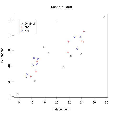
When you have more than one set of data you may want to bring them
together. You can bring different data sets together by appending as
rows (rbind) or by appending as columns (cbind). The first example
shows how this done with two data frames. The arguments to the
functions can take any number of objects. We only use two here to keep
the demonstration simpler, but additional data frames can be appended
in the same call. It is important to note that when you bring things
together as rows the names of the objects within the data frame must
be the same.
> a <- data.frame(one=c( 0, 1, 2),two=c("a","a","b"))
> b <- data.frame(one=c(10,11,12),two=c("c","c","d"))
> a
one two
1 0 a
2 1 a
3 2 b
> b
one two
1 10 c
2 11 c
3 12 d
> v <- rbind(a,b)
> typeof(v)
[1] "list"
> v
one two
1 0 a
2 1 a
3 2 b
4 10 c
5 11 c
6 12 d
> w <- cbind(a,b)
> typeof(w)
[1] "list"
> w
one two one two
1 0 a 10 c
2 1 a 11 c
3 2 b 12 d
> names(w) = c("one","two","three","four")
> w
one two three four
1 0 a 10 c
, .toc-backref2 1 a 11 c
3 2 b 12 d
The same commands also work with vectors and matrices and behave in a similar manner.
> A = matrix(c( 1, 2, 3, 4, 5, 6),ncol=3,byrow=TRUE)
> A
[,1] [,2] [,3]
[1,] 1 2 3
[2,] 4 5 6
> B = matrix(c(10,20,30,40,50,60),ncol=3,byrow=TRUE)
> B
[,1] [,2] [,3]
[1,] 10 20 30
[2,] 40 50 60
> V <- rbind(A,B)
> typeof(V)
[1] "double"
> V
[,1] [,2] [,3]
[1,] 1 2 3
[2,] 4 5 6
[3,] 10 20 30
[4,] 40 50 60
> W <- cbind(A,B)
> typeof(W)
[1] "double"
> W
[,1] [,2] [,3] [,4] [,5] [,6]
[1,] 1 2 3 10 20 30
[2,] 4 5 6 40 50 60
The various apply functions can be an invaluable tool when trying to
work with subsets within a data set. The different versions of the
apply commands are used to take a function and have the function
perform an operation on each part of the data. There are a wide
variety of these commands, but we only look at two sets of them. The
first set, lapply and sapply, is used to apply a function to every
element in a list. The second one, tapply, is used to apply a
function on each set broken up by a given set of factors.
13.2.1. Operations on Lists and Vectors
First, the lapply command is used to take a list of items and
perform some function on each member of the list. That is, the list
includes a number of different objects. You want to perform some
operation on every object within the list. You can use lapply to
tell R to go through each item in the list and perform the desired
action on each item.
In the following example a list is created with three elements. The
first is a randomly generated set of numbers with a normal
distribution. The second is a randomly generated set of numbers with
an exponential distribution. The last is a set of factors. A summary
is then performed on each element in the list.
> x <- list(a=rnorm(200,mean=1,sd=10),
b=rexp(300,10.0),
c=as.factor(c("a","b","b","b","c","c")))
> lapply(x,summary)
$a
Min. 1st Qu. Median Mean 3rd Qu. Max.
-26.65000 -6.91200 -0.39250 0.09478 6.86700 32.00000
$b
Min. 1st Qu. Median Mean 3rd Qu. Max.
0.0001497 0.0242300 0.0633300 0.0895400 0.1266000 0.7160000
$c
a b c
1 3 2
The lapply command returns a list. The entries in the list have the
same names as the entries in the list that is passed to it. The values
of each entry are the results from applying the function. The sapply
function is similar, but the difference is that it tries to turn
the result into a vector or matrix if possible. If it does not make
sense then it returns a list just like the lapply command.
> x <- list(a=rnorm(8,mean=1,sd=10),b=rexp(10,10.0))
> x
$a
[1] -0.3881426 6.2910959 13.0265859 -1.5296377 6.9285984 -28.3050569
[7] 11.9119731 -7.6036997
$b
[1] 0.212689007 0.081818395 0.222462531 0.181424705 0.168476454 0.002924134
[7] 0.007010114 0.016301837 0.081291728 0.055426055
> val <- lapply(x,mean)
> typeof(val)
[1] "list"
> val
$a
[1] 0.04146456
$b
[1] 0.1029825
> val$a
[1] 0.04146456
> val$b
[1] 0.1029825
>
>
> other <- sapply(x,mean)
> typeof(other)
[1] "double"
> other
a b
0.04146456 0.10298250
> other[1]
a
0.04146456
> other[2]
b
0.1029825
13.2.2. Operations By Factors
Another widely used variant of the apply functions is the tapply
function. The tapply function will take a list of data, usually a vector, a list of factors of the same list, and a function. It will then apply the function to each subset of the data that matches each of the factors.
> val <- data.frame(a=c(1,2,10,20,5,50),
b=as.factor(c("a","a","b","b","a","b")))
> val
a b
1 1 a
2 2 a
3 10 b
4 20 b
5 5 a
6 50 b
> result <- tapply(val$a,val$b,mean)
> typeof(result)
[1] "double"
> result
a b
2.666667 26.666667
> result[1]
a
2.666667
, .toc-backref> result[2]
b
26.66667
> result <- tapply(val$a,val$b,summary)
> typeof(result)
[1] "list"
> result
$a
Min. 1st Qu. Median Mean 3rd Qu. Max.
1.000 1.500 2.000 2.667 3.500 5.000
$b
Min. 1st Qu. Median Mean 3rd Qu. Max.
10.00 15.00 20.00 26.67 35.00 50.00
> result$a
Min. 1st Qu. Median Mean 3rd Qu. Max.
1.000 1.500 2.000 2.667 3.500 5.000
> result$b
Min. 1st Qu. Median Mean 3rd Qu. Max.
10.00 15.00 20.00 26.67 35.00 50.00
14. Time Data Types
The time data types are broken out into a separate section from the
introductory section on data types. (Basic Data Types) The reason
for this is that dealing with time data can be subtle and must be done
carefully because the data type can be cast in a variety of different
ways. It is not an introductory topic, and if not done well can scare
off the normal people.
I will first go over the basic time data types and then explore the
different kinds of operations that are done with the time data
types. Please be cautious with time data and read the complete
description including the caveats. There are some common mistakes that
result in calculations that yield results that are very different from
the intended values.
There are a variety of different types specific to time data fields
in R. Here we only look at two, the POSIXct and POSIXlt data types:
POSIXct
The POSIXct data type is the number of seconds since the start
of January 1, 1970. Negative numbers represent the number of seconds
before this time, and positive numbers represent the number of
seconds afterwards.
POSIXlt
The POSIXlt data type is a vector, and the entries in the vector
have the following meanings:
- seconds
- minutes
- hours
- day of month (1-31)
- month of the year (0-11)
- years since 1900
- day of the week (0-6 where 0 represents Sunday)
- day of the year (0-365)
- Daylight savings indicator (positive if it is daylight savings)
Part of the difficulty with time data types is that R prints them out
in a way that is different from how it stores them internally. This
can make type conversions tricky, and you have to be careful and test
your operations to insure that R is doing what you think it is doing.
To get the current time, the Sys.time() can be used, and you can
play around a bit with the basic types to get a feel for what R is
doing. The as.POSIXct and as.POSIXlt commands are used to
convert the time value into the different formats.
> help(DateTimeClasses)
> t <- Sys.time()
> typeof(t)
[1] "double"
> t
[1] "2014-01-23 14:28:21 EST"
> print(t)
[1] "2014-01-23 14:28:21 EST"
> cat(t,"\n")
1390505301
> c <- as.POSIXct(t)
> typeof(c)
[1] "double"
> print(c)
[1] "2014-01-23 14:28:21 EST"
> cat(c,"\n")
1390505301
>
>
> l <- as.POSIXlt(t)
> l
[1] "2014-01-23 14:28:21 EST"
> typeof(l)
[1] "list"
> print(l)
[1] "2014-01-23 14:28:21 EST"
> cat(l,"\n")
Error in cat(list(...), file, sep, fill, labels, append) :
argument 1 (type 'list') cannot be handled by 'cat'
> names(l)
NULL
> l[[1]]
[1] 21.01023
> l[[2]]
[1] 28
> l[[3]]
[1] 14
> l[[4]]
[1] 23
> l[[5]]
[1] 0
> l[[6]]
[1] 114
> l[[7]]
[1] 4
> l[[8]]
[1] 22
> l[[9]]
[1] 0
>
> b <- as.POSIXct(l)
> cat(b,"\n")
1390505301
There are times when you have a time data type and want to convert it
into a string so it can be saved into a file to be read by another
application. The strftime command is used to take a time data type
and convert it to a string. You must supply an additional format
string to let R what format you want to use. See the help page on
strftime to get detailed information about the format string.
> help(strftime)
>
> t <- Sys.time()
> cat(t,"\n")
1390506463
> timeStamp <- strftime(t,"%Y-%m-%d %H:%M:%S")
> timeStamp
[1] "2014-01-23 14:47:43"
> typeof(timeStamp)
[1] "character"
Commonly a time stamp is saved in a data file, and it must be
converted into a time data type to allow for calculations. For
example, you may be interested in how much time has elapsed between
two observations. The strptime command is used to take a string and
convert it into a time data type. Like strftime it requires a format
string in addition to the time stamp.
The strptime command is used to take a string and convert it into a
form that R can use for calculations. In the following example a data
frame is defined that has the dates stored as strings. If you read the
data in from a csv file this is how R will keep track of the
data. Note that in this context the strings are assumed to represent
ordinal data, and R will assume that the data field is a set of
factors. You have to use the strptime command to convert it into a
time field.
> myData <- data.frame(time=c("2014-01-23 14:28:21","2014-01-23 14:28:55",
"2014-01-23 14:29:02","2014-01-23 14:31:18"),
speed=c(2.0,2.2,3.4,5.5))
> myData
time speed
1 2014-01-23 14:28:21 2.0
2 2014-01-23 14:28:55 2.2
3 2014-01-23 14:29:02 3.4
4 2014-01-23 14:31:18 5.5
> summary(myData)
time speed
2014-01-23 14:28:21:1 Min. :2.000
2014-01-23 14:28:55:1 1st Qu.:2.150
2014-01-23 14:29:02:1 Median :2.800
2014-01-23 14:31:18:1 Mean :3.275
3rd Qu.:3.925
Max. :5.500
> myData$time[1]
[1] 2014-01-23 14:28:21
4 Levels: 2014-01-23 14:28:21 2014-01-23 14:28:55 ... 2014-01-23 14:31:18
> typeof(myData$time[1])
[1] "integer"
>
>
> myData$time <- strptime(myData$time,"%Y-%m-%d %H:%M:%S")
> myData
time speed
1 2014-01-23 14:28:21 2.0
2 2014-01-23 14:28:55 2.2
3 2014-01-23 14:29:02 3.4
4 2014-01-23 14:31:18 5.5
> myData$time[1]
[1] "2014-01-23 14:28:21"
> typeof(myData$time[1])
[1] "list"
> myData$time[1][[2]]
[1] 28
Now you can perform operations on the fields. For example you can
determine the time between observations. (Please see the notes below
on time operations. This example is a bit misleading!)
> N = length(myData$time)
> myData$time[2:N] - myData$time[1:(N-1)]
Time differences in secs
[1] 34 7 136
attr(,"tzone")
[1] ""
In addition to the time data types R also has a date data type. The
difference is that the date data type keeps track of numbers of days
rather than seconds. You can cast a string into a date type using the
as.Date function. The as.Date function takes the same arguments as
the time data types discussed above.
> theDates <- c("1 jan 2012","1 jan 2013","1 jan 2014")
> dateFields <- as.Date(theDates,"%d %b %Y")
> typeof(dateFields)
[1] "double"
> dateFields
[1] "2012-01-01" "2013-01-01" "2014-01-01"
> N <- length(dateFields)
> diff <- dateFields[1:(N-1)] - dateFields[2:N]
> diff
Time differences in days
[1] -366 -365
You can also define a date in terms of the number days after another
date using the origin option.
> infamy <- as.Date(-179,origin="1942-06-04")
> infamy
[1] "1941-12-07"
>
> today <- Sys.Date()
> today
[1] "2014-01-23"
> today-infamy
Time difference of 26345 days
Finally, a nice function to know about and use is the format
command. It can be used in a wide variety of situations, and not just
for dates. It is helpful for dates, though, because you can use it in
cat and print statements to make sure that your output is in
exactly the form that you want.
> theTime <- Sys.time()
> theTime
[1] "2014-01-23 16:15:05 EST"
> a <- rexp(1,0.1)
> a
[1] 7.432072
> cat("At about",format(theTime,"%H:%M"),"the time between occurances was around",format(a,digits=3),"seconds\n")
At about 16:15 the time between occurances was around 7.43 seconds
The most difficult part of dealing with time data can be converting it
into the right format. Once a time or date is stored in R’s internal
format then a number of basic operations are available. The thing to
keep in mind, though, is that the units you get after an operation can
vary depending on the magnitude of the time values. Be very careful
when dealing with time operations and vigorously test your codes.
> now <- Sys.time()
> now
[1] "2014-01-23 16:31:00 EST"
> now-60
[1] "2014-01-23 16:30:00 EST"
>
> earlier <- strptime("2000-01-01 00:00:00","%Y-%m-%d %H:%M:%S")
> later <- strptime("2000-01-01 00:00:20","%Y-%m-%d %H:%M:%S")
> later-earlier
Time difference of 20 secs
> as.double(later-earlier)
[1] 20
>
> earlier <- strptime("2000-01-01 00:00:00","%Y-%m-%d %H:%M:%S")
> later <- strptime("2000-01-01 01:00:00","%Y-%m-%d %H:%M:%S")
> later-earlier
Time difference of 1 hours
> as.double(later-earlier)
[1] 1
>
> up <- as.Date("1961-08-13")
> down <- as.Date("1989-11-9")
> down-up
Time difference of 10315 days
The two examples involving the variables earlier and later in the
previous code sample should cause you a little concern. The value of
the difference depends on the largest units with respect to the
difference! The issue is that when you subtract dates R uses the
equivalent of the difftime command. We need to know how this
operates to reduce the ambiguity when comparing times.
> help(difftime)
>
> earlier <- strptime("2000-01-01 00:00:00","%Y-%m-%d %H:%M:%S")
> later <- strptime("2000-01-01 01:00:00","%Y-%m-%d %H:%M:%S")
> difftime(later,earlier)
Time difference of 1 hours
> difftime(later,earlier,units="secs")
Time difference of 3600 secs
One thing to be careful about difftime is that it is a double
precision number, but it has units attached to it. This can be tricky,
and you should be careful about the ambiguity in using this command. I
personally always try to specify the units to avoid this.
> earlier <- strptime("2000-01-01 00:00:00","%Y-%m-%d %H:%M:%S")
> later <- strptime("2000-01-01 00:00:20","%Y-%m-%d %H:%M:%S")
> d <- difftime(later,earlier)
> d
Time difference of 20 secs
> typeof(d)
[1] "double"
> as.double(d)
[1] 20
Another way to define a time difference is to use the as.difftime
command. It takes two dates and will compute the difference between
them. It takes a time, its format, and the units to use. Note that in
the following example R is able to figure out what the units are when
making the calculation.
> diff <- as.difftime("00:30:00","%H:%M:%S",units="hour")
> diff
Time difference of 0.5 hours
> Sys.time()
[1] "2014-01-23 16:45:39 EST"
> Sys.time()+diff
[1] "2014-01-23 17:15:41 EST"
The last thing to mention is that once a time stamp is cast into one
of R’s internal formats comparisons can be made in a natural way.
> diff <- as.difftime("00:30:00","%H:%M:%S",units="hour")
> now <- Sys.time()
> later <- now + diff
> now
, .toc-backref[1] "2014-01-23 16:47:48 EST"
> later
[1] "2014-01-23 17:17:48 EST"
>
> if(now < later)
{
cat("there you go\n")
}
there you go
15. Introduction to Programming
We look at running commands from a source file. We also include an
overview of the different statements that are used for control-flow
that determines which code is executed by the interpreter.
In the next section the ways to execute the commands in a file using
the source command are given. The remaining sections are used to
list the various flow control options that are available in the R
language definition. The language definition has a wide variety of
control functions which can be found using the help command.
A set of R commands can be saved in a file and then executed as if you
had typed them in from the command line. The source command is used
to read the file and execute the commands in the same sequence given
in the file.
> source('file.R')
> help(source)
>
If you simply source the file the commands are not printed, and the
results of commands are not printed. This can be overridden using the
echo, print.eval, and verbose options.
Some examples are given assuming that a file, simpleEx.R, is in the
current directory. The file is given below:
# Define a variable.
x <- rnorm(10)
# calculate the mean of x and print out the results.
mux = mean(x)
cat("The mean of x is ",mean(x),"\n")
# print out a summary of the results
summary(x)
cat("The summary of x is \n",summary(x),"\n")
print(summary(x))
The file also demonstrates the use of # to specify
comments. Anything after the # is ignored. Also, the file
demonstrates the use of cat and print to send results to the
standard output. Note that the commands have options to send results
to a file. Use help for more information.
The output for the different options can be found below:
> source('simpleEx.R')
The mean of x is -0.4817475
The summary of x is
-2.24 -0.5342 -0.2862 -0.4817 -0.1973 0.4259
Min. 1st Qu. Median Mean 3rd Qu. Max.
-2.2400 -0.5342 -0.2862 -0.4817 -0.1973 0.4259
>
>
>
> source('simpleEx.R',echo=TRUE)
Min. 1st Qu. Median Mean 3rd Qu. Max.
-2.32600 -0.69140 -0.06772 -0.13540 0.46820 1.69600
>
>
>
> source('simpleEx.R',print.eval=TRUE)
The mean of x is 0.1230581
Min. 1st Qu. Median Mean 3rd Qu. Max.
-1.7020 -0.2833 0.1174 0.1231 0.9103 1.2220
The summary of x is
-1.702 -0.2833 0.1174 0.1231 0.9103 1.222
Min. 1st Qu. Median Mean 3rd Qu. Max.
-1.7020 -0.2833 0.1174 0.1231 0.9103 1.2220
>
>
>
> source('simpleEx.R',print.eval=FALSE)
The mean of x is 0.6279428
The summary of x is
-0.7334 -0.164 0.9335 0.6279 1.23 1.604
Min. 1st Qu. Median Mean 3rd Qu. Max.
-0.7334 -0.1640 0.9335 0.6279 1.2300 1.6040
>
>
>
>
> source('simpleEx.R',verbose=TRUE)
'envir' chosen:<environment: R_GlobalEnv>
encoding = "native.enc" chosen
--> parsed 6 expressions; now eval(.)ing them:
>>>> eval(expression_nr. 1 )
=================
> # Define a variable.
> x <- rnorm(10)
curr.fun: symbol <-
.. after ‘expression(x <- rnorm(10))’
>>>> eval(expression_nr. 2 )
=================
> # calculate the mean of x and print out the results.
> mux = mean(x)
curr.fun: symbol =
.. after ‘expression(mux = mean(x))’
>>>> eval(expression_nr. 3 )
=================
> cat("The mean of x is ",mean(x),"\n")
The mean of x is -0.1090932
curr.fun: symbol cat
.. after ‘expression(cat("The mean of x is ",mean(x),"\n"))’
>>>> eval(expression_nr. 4 )
=================
> # print out a summary of the results
> summary(x)
curr.fun: symbol summary
Min. 1st Qu. Median Mean 3rd Qu. Max.
-1.3820 -1.0550 -0.1995 -0.1091 0.6813 2.1050
.. after ‘expression(summary(x))’
>>>> eval(expression_nr. 5 )
=================
> cat("The summary of x is \n",summary(x),&q, .toc-backrefuot;\n")
The summary of x is
-1.382 -1.055 -0.1995 -0.1091 0.6813 2.105
curr.fun: symbol cat
.. after ‘expression(cat("The summary of x is \n",summary(x),"\n"))’
>>>> eval(expression_nr. 6 )
=================
> print(summary(x))
Min. 1st Qu. Median Mean 3rd Qu. Max.
-1.3820 -1.0550 -0.1995 -0.1091 0.6813 2.1050
curr.fun: symbol print
.. after ‘expression(print(summary(x)))’
One common problem that occurs is that R may not know where to find a
file.
> source('notThere.R')
Error in file(filename, "r", encoding = encoding) :
cannot open the connection
In addition: Warning message:
In file(filename, "r", encoding = encoding) :
cannot open file 'notThere.R': No such file or directory
R will search the current working directory. You can see what files
are in the directory using the dir command, and you can determine
the current directory using the getwd command.
> getwd()
[1] "/home/black/public_html/tutorial/R/rst/source/R"
> dir()
[1] "plotting.rData" "power.R" "shadedRegion.R"
You can change the current directory, and the options available depend
on how you are using R. For example on a Windows PC or a Macintosh you
can use the menu options to change the working directory. You can
choose the directory using a graphical file browser. Otherwise, you
can change to the correct directory before running R or use the
setwd command.
Conditional execution is available using the if statement and the
corresponding else statement.
> x = 0.1
> if( x < 0.2)
{
x <- x + 1
cat("increment that number!\n")
}
, .toc-backrefincrement that number!
> x
[1] 1.1
The else statement can be used to specify an alternate option. In the
example below note that the else statement must be on the same line
as the ending brace for the previous if block.
> x = 2.0
> if ( x < 0.2)
{
x <- x + 1
cat("increment that number!\n")
} else
{
x <- x - 1
cat("nah, make it smaller.\n");
}
nah, make it smaller.
> x
[1] 1
Finally, the if statements can be chained together for multiple
options. The if statement is considered a single code block, so more
if statements can be added after the else.
> x = 1.0
> if ( x < 0.2)
{
x <- x + 1
cat("increment that number!\n")
} else if ( x < 2.0)
{
x <- 2.0*x
cat("not big enough!\n")
} else
{
x <- x - 1
, .toc-backref cat("nah, make it smaller.\n");
}
not big enough!
> x
[1] 2
The argument to the if statement is a logical expression. A full
list of logical operators can be found in the types document focusing
on logical variables (Logical).
The for loop can be used to repeat a set of instructions, and it is
used when you know in advance the values that the loop variable will
have each time it goes through the loop. The basic format for the
for loop is for(var in seq) expr
An example is given below:
> for (lupe in seq(0,1,by=0.3))
{
cat(lupe,"\n");
}
0
0.3
0.6
0.9
>
> x <- c(1,2,4,8,16)
> for (loop in x)
{
cat("value of loop: ",loop,"\n");
}
value of loop: 1
value of loop: 2
value of loop: 4
value of loop: 8
value of loop: 16
See the section on breaks for more options (break and next statements)
The while loop can be used to repeat a set of instructions, and, .toc-backref it
is often used when you do not know in advance how often the
instructions will be executed. The basic format for a while loop is
while(cond) expr
>
> lupe <- 1;
> x <- 1
> while(x < 4)
{
x <- rnorm(1,mean=2,sd=3)
cat("trying this value: ",x," (",lupe," times in loop)\n");
lupe <- lupe + 1
}
trying this value: -4.163169 ( 1 times in loop)
trying this value: 3.061946 ( 2 times in loop)
trying this value: 2.10693 ( 3 times in loop)
trying this value: -2.06527 ( 4 times in loop)
trying this value: 0.8873237 ( 5 times in loop)
trying this value: 3.145076 ( 6 times in loop)
trying this value: 4.504809 ( 7 times in loop)
See the section on breaks for more options (break and next statements)
The repeat loop is similar to the while loop. The difference is
that it will always begin the loop the first time. The while loop
will only start the loop if the condition is true the first time it is
evaluated. Another difference is that you have to explicitly specify
when to stop the loop using the break command.
That is you need to execute the break statement to get out of the
loop.
> repeat
{
x <- rnorm(1)
if(x < -2.0) break
}
> x
[1] -2.300532
See the section on breaks for more options (break and next statements)
The break statement is used to stop the execution of the current
loop. It will break out of the current loop. The next statement is
used to skip the statements that follow and restart the current
loop. If a for loop is used then the next statement will update
the loop variable.
> x <- rnorm(5)
> x
[1] 1.41699338 2.28086759 -0.01571884 0.56578443 0.60400784
> for(lupe in x)
{
if (lupe > 2.0)
next
if( (lupe<0.6) && (lupe > 0.5))
break
cat("The value of lupe is ",lupe,"\n");
}
The value of lupe is 1.416993
The value of lupe is -0.01571884
The switch takes an expression and returns a value in a list based
on the value of the expression. How it does this depends on the data
type of the expression. The basic syntax is switch(statement,item1,item2,item3,...,itemN).
If the result of the expression is a number then it returns the item
in the list with the same index. Note that the expression is cast as
an integer if it is not an integer.
> x <- as.integer(2)
> x
[1] 2
> z = switch(x,1,2,3,4,5)
> z
[1] 2
> x <- 3.5
> z = switch(x,1,2,3,4,5)
> z
[1] 3
If the result of the expression is a string, then the list of items
should be in the form “valueN”=resultN, and the statement will
return the result that matches the value.
> y <- rnorm(5)
> y
[1] 0.4218635 -0.8205637 -1.0191267 -0.6080061 -0.6079133
> x <- "sd"
> z <- switch(x,"mean"=mean(y),"median"=median(y),"variance"=var(y),"sd"=sd(y))
> z
[1] 0.5571847
> x <- "median"
> z <- switch(x,"mean"=mean(y),"median"=median(y),"variance"=var(y),"sd"=sd(y))
> z
[1] -0.6080061
The command to read input from the keyboard is the scan
statement. It has a wide variety of options and can be fine tuned to
your specific needs. We only look at the basics here. The scan
statement waits for input from a user, and it returns the value that
was typed in.
When using the command with no set number of lines the command will
continue to read keyboard input until a blank line is entered.
> help(scan)
> a <- scan(what=double(0))
1: 3.5
2:
Read 1 item
> a
[1] 3.5
> typeof(a)
[1] "double"
>
> a <- scan(what=double(0))
1: yo!
1:
Error in scan(file, what, nmax, sep, dec, quote, skip, nlines, na.strings, :
scan() expected 'a real', got 'yo!'
If you wish to only have it read from a fixed number of lines the
nmax option can specify how many lines can be typed in, and the
multi.line option can be used to turn off multi-line entry.
> a <- scan(what=double(0),nmax=1,multi.line = FALSE)
1: 6.7
Read 1 item
> a
[1] 6.7
A shallow overview of defining functions is given here. A few
subtleties will be noted, but R can be a little quirky with respect to
defining functions. The first bit of oddness is that you can think of
a function as an object where you define the function and assign it to
a variable name.
To define a function you assign it to a name, and the keyword
function is used to denote the start of the function and its
argument list.
> newDef <- function(a,b)
{
x = runif(10,a,b)
mean(x)
}
> newDef(-1,1)
[1] 0.06177728
> newDef
function(a,b)
{
x = runif(10,a,b)
mean(x)
}
The last expression in the function is what is returned. So in the
example above the sample mean of the numbers is returned.
> x <- newDef(0,1)
> x
[1] 0.4800442
The arguments that are passed are matched in order. They can be
specified explicitly, though.
> newDef(b=10,a=1)
[1] 4.747509
> newDef(10,1)
[1] NaN
Warning message:
In runif(10, a, b) : NAs produced
You can mix this approach, and R will try to match up the named
arguments and then match the rest going from left to right. Another
bit of weirdness is that R will not evaluate an expression in the
argument list until the moment it is needed in the function. This is a
different kind of behavior than what most people are used to, so be
very careful about this. The best rule of thumb is to not put in
operations in an argument list if they matter after the function is
called.
Another common task is to have a function return multiple items. This
can be accomplished by returning a list of items. The objects within
a list can be accessed using the same $ notation that is used for
data frames.
> c = c(1,2,3,4,5)
> sample <- function(a,b)
{
value = switch(a,"median"=median(b),"mean"=mean(b),"variance"=var(b))
largeVals = length(c[c>1])
list(stat=value,number=largeVals)
}
> result <- sample("median",c)
> result
$stat
[1] 3
$number
[1] 4
> result$stat
[1] 3
> result$number
[1] 4
There is another potential problem that can occur when using a
function in R. When it comes to determining the value of a variable
there is a path that R will use to search for its value. In the case
of functions if a previously undefined variable appears R will look at
the argument list for the function. Next it will look in the current
work space. If you are not careful R will find the value some place
where you do not expect it, and your function will return a value that
is not correct, and no error will be given. Be very careful about the
names of variables especially when using functions.
Object Oriented Programming
There are at least three different approaches to object oriented programming in R. We examine two of them, the S3 and S4 classes. The other approach makes use of a package, and we focus instead on the two built in classes.
1. S3 Classes
We examine how to create S3 classes. It is assumed that you are familiar with the basic data types and scripting (Introduction to Programming).
First, everything in R is treated like as an object. We have seen this with functions. Many of the objects that are created within an R session have attributes associated with them. One common attribute associated with an object is its class.
You can set the class attribute using the class command. One thing to notice is that the class is a vector which allows an object to inherit from multiple classes, and it allows you to specify the order of inheritance for complex classes. You can also use the class command to determine the classes associated with an object.
> bubba <- c(1,2,3)
> bubba
[1] 1 2 3
>
> class(bubba)
[1] "numeric"
>
> class(bubba) <- append(class(bubba),"Flamboyancy")
> class(bubba)
[1] "numeric" "Flamboyancy"
Note
A new command, append, is used here. The first argument is a vector, and the function adds the following arguments to the end of the vector.
One way to define a method for a class is to use the UseMethod command to define a hierarchy of functions that will react appropriately. The UseMethod command will tell R to look for a function whose prefix matches the current function, and it searches for a suffix in order from the vector of class names. In other words a set of functions can be defined, and the function that is actually called will be determined by the class name of the first object in the list of arguments.
You first have, .toc-backref to define a generic function to reserve the function name. The UseMethod command is then used to tell the R system to search for a different function. The search is based on the name of the function and the names of an object’s classes. The name of the functions have two parts separated by a ”.” where the prefix is the function name and the suffix is the name of a class.
That is a lot of verbiage 罗嗦 to describe a relatively simple idea. A very basic example is given below:
> bubba <- list(first="one", second="two", third="third")
> class(bubba) <- append(class(bubba),"Flamboyancy")
>
> bubba
$first
[1] "one"
$second
[1] "two"
$third
[1] "third"
attr(,"class")
[1] "list" "Flamboyancy"
>
> GetFirst <- function(x)
+ {
+ UseMethod("GetFirst",x)
+ }
>
> GetFirst.Flamboyancy <- function(x)
+ {
+ return(x$first)
+ }
>
> GetFirst(bubba)
[1] "one"
The plethora of object oriented approaches leads to a natural
question. Which one should you use? With respect to S3 and S4 classes,
the S3 class is more flexible, and the S4 class is a more structured
approach. This is a nice way of saying that the S3 class approach is
for unaware slobs and is a sloppy way to shoot yourself in the foot,
while the S4 class is for uptight pedants.
Our focus here is on S3 classes. Before we delve into the details of
S3 classes we need to talk about memory environments. These can be
used to great effect in S3 classes to make your codes totally
incomprehensible. On the down side they help give S3 classes their
flexibility.
An environment can be thought of as a local scope. It has a set of
variables associa, .toc-backrefted with it. You can access those variables if you
have the “ID’’ associated with the environment. There are a number of
commands you can use to manipulate and obtain the pointers to your
environments. You can also use the assign and get commands to set
and get the values of variables within an environment.
The environment command can be used to get the pointer to the
current environment.
> ls()
character(0)
> e <- environment()
> e
<environment: R_GlobalEnv>
> assign("bubba",3,e)
> ls()
[1] "bubba" "e"
> bubba
[1] 3
> get("bubba",e)
[1] 3
Environments can be created and embedded within other environments and
can be structured to form a hierarchy. There are a number of commands
to help you move through different environments. You can find more
details using the command help(environment), but we do not pursue
more details because this is as much as we need for our purposes of
using S3 classes.
The basic ideas associated with S3 classes is discussed in the first
section (The Basic Idea). We now expand on that idea and
demonstrate how to define a function that will create and return an
object of a given class. The basic idea is that a list is created with
the relevant members, the list’s class is set, and a copy of the list
is returned.
Here we examine two different ways to construct an S3 class. The first
approach is more commonly used and is more straightforward. It makes
use of basic list properties. The second approach makes use of the
local environment within a function to define the variables tracked by
the class. The advantage to the second approach is that it looks more
like the object oriented approach that many are familiar with. The
disadvantage is that it is more difficult to read the code, and it is
more like working with pointers which is different from the way other
objects work in R.
The first approach is the more standard approach most often seen with
S3 classes. It makes use of the methods defined outside of the class
which is described below, Creating Methods. It also keeps track
of the data maintained by the class using the standard practices
associated with lists.
The basic idea is that a function is defined which creates a list. The
data entries tracked by the class are defined in the list. In the
example below the defaults are specified in the argument list with
default values assigned. A new class name is appended to the list’s
classes, and the list is returned.
NorthAmerican <- function(eatsBreakfast=TRUE,myFavorite="cereal")
{, .toc-backref
me <- list(
hasBreakfast = eatsBreakfast,
favoriteBreakfast = myFavorite
)
## Set the name for the class
class(me) <- append(class(me),"NorthAmerican")
return(me)
}
Once this definition is executed a new function is defined, called
NorthAmerican. A new object of this class can be created by calling
the function.
> bubba <- NorthAmerican()
> bubba
$hasBreakfast
[1] TRUE
$favoriteBreakfast
[1] "cereal"
attr(,"class")
[1] "list" "NorthAmerican"
> bubba$hasBreakfast
[1] TRUE
>
> louise <- NorthAmerican(eatsBreakfast=TRUE,myFavorite="fried eggs")
> louise
$hasBreakfast
[1] TRUE
$favoriteBreakfast
[1] "fried eggs"
attr(,"class")
[1] "list" "NorthAmerican"
Another approach can be employed that makes use of the local
environment within a function to access the variables. When we define
methods with this approach later, Local Environment Approach, the
results will look more like object oriented approaches seen in other
languages.
The approach relies on the local scope created when a function is
called. A new environment is created that can be identified using the
environment command. The environment can be saved in the list
created for the class, and the variables within this scope can then be
accessed using the identification of the environment.
In the example below this approach appears to require more
overhead. When we examine how to add external methods to the class the
advantage will be a little clearer.
NordAmericain <- function(eatsBreakfast=TRUE,myFavorite="cereal")
{
## Get the environment for this
## instance of the function.
thisEnv <- environment()
hasBreakfast <- eatsBreakfast
favoriteBreakfast <- myFavorite
## Create the list used to represent an
## object for this class
me <- list(
## Define the environment where this list is defined so
## that I can refer to it later.
thisEnv = thisEnv,
## The Methods for this class normally go here but are discussed
## below. A simple placeholder is here to give you a teaser....
getEnv = function()
{
return(get("thisEnv",thisEnv))
}
)
## Define the value of the list within the current environment.
assign('this',me,envir=thisEnv)
## Set the name for the class
class(me) <- append(class(me),"NordAmericain")
return(me)
}
Now that the class is defined, the environment used for a given object
can be easily retrieved.
> bubba <- NordAmericain()
> get("hasBreakfast",bubba$getEnv())
[1] TRUE
> get("favoriteBreakfast",bubba$getEnv())
[1] "cereal"
Note that there is an unfortunate side effect to this approach. By
keeping track of the environment, it is similar to using a pointer to
the variables rather than the variables themselves. This means when
you make a copy, you are making a copy of the pointer to the
environment.
> bubba <- NordAmericain(myFavorite="oatmeal")
> get("favoriteBreakfast",bubba$getEnv())
[1] "oatmeal"
> louise <- bubba
> assign("favoriteBreakfast","toast",louise$getEnv())
> get("favoriteBreakfast",louise$getEnv())
[1] "toast"
> get("favoriteBreakfast",bubba$getEnv())
[1] "toast"
This issue will be explored again in the subsection below detailing
how to create methods for an S3 class. If you wish to be able to copy
an object using this approach you need to create a new method to
return a proper copy.
We now explore how to create methods associated with a class. Again we
break it up into two parts. The first approach is used for both
approaches discussed in the previous section. If you make use of the
local environment approach discussed above you will likely make use of
both approaches discussed in this section. If you only make use of the
more straight forward approach you only need to be aware of the first
approach discussed here.
The first approach is to define a function that exists outside of the
class. The function is defined in a generic way, and then a function
specific to a given class is defined. The R environment then decides
which function to use based on the class names of an argument to the
function, and the suffix used in the names of the associated
functions.
One thing to keep in mind is that for assignment R makes copies of
objects. The implication is that if you change a part of an object you
need to return an exact copy of the object. Otherwise your changes may
be lost.
In the examples below we define accessors for the variables in the
class defined above. We assume that the class NorthAmerican is
defined in the same way as the first example above,
Straightforward Class. In the first
example the goal is that we want to create a function that will set
the value of hasBreakfast for a given object. The name of the
function will be setHasBreakfast.
The first step is to reserve the name of the function, and use the
UseMethod command to tell R to search for the correct function. If
we pass an object whose class includes the name NorthAmerican then
the correct function to call should be called
setHasBreakfast.NorthAmerican. Note that we will also create a
function called setHasBreakfast.default. This function will be
called if R cannot find another function of the correct class.
setHasBreakfast <- function(elObjeto, newValue)
{
print("Calling the base setHasBreakfast function")
UseMethod("setHasBreakfast",elObjeto)
print("Note this is not executed!")
}
setHasBreakfast.default <- function(elObjeto, newValue)
{
print("You screwed up. I do not know how to handle this object.")
return(elObjeto)
}
setHasBreakfast.NorthAmerican <- function(elObjeto, newValue)
{
print("In setHasBreakfast.NorthAmerican and setting the value")
elObjeto$hasBreakfast <- newValue
return(elObjeto)
}
The first thing to note is that the function returns a copy of the
object passed to it. R passes copies of objects to functions. If you
change an object within a function it does not change the original
object. You must pass back a copy of the updated object.
> bubba <- NorthAmerican()
> bubba$hasBreakfast
[1] TRUE
> bubba <- setHasBreakfast(bubba,FALSE)
[1] "Calling the base setHasBreakfast function"
[1] "In setHasBreakfast.NorthAmerican and setting the value"
> bubba$hasBreakfast
[1] FALSE
> bubba <- setHasBreakfast(bubba,"No type checking sucker!")
[1] "Calling the base setHasBreakfast function"
[1] "In setHasBreakfast.NorthAmerican and setting the value"
> bubba$hasBreakfast
[1] "No type checking sucker!"
If the correct function cannot be found then the default version of
the function is called.
> someNumbers <- 1:4
> someNumbers
[1] 1 2 3 4
> someNumbers <- setHasBreakfast(someNumbers,"what?")
[1] "Calling the base setHasBreakfast function"
[1] "You screwed up. I do not know how to handle this object."
> someNumbers
[1] 1 2 3 4
It is a good practice to only use predefined accessors to get and set
values held by an object. As a matter of completeness we define
methods to get the value of the hasBreakfast field.
getHasBreakfast <- function(elObjeto)
{
<, .toc-backrefspan class="kp">print("Calling the base getHasBreakfast function")
UseMethod("getHasBreakfast",elObjeto)
print("Note this is not executed!")
}
getHasBreakfast.default <- function(elObjeto)
{
print("You screwed up. I do not know how to handle this object.")
return(NULL)
}
getHasBreakfast.NorthAmerican <- function(elObjeto)
{
print("In getHasBreakfast.NorthAmerican and returning the value")
return(elObjeto$hasBreakfast)
}
The functions to get the values are used in the same way.
> bubba <- NorthAmerican()
> bubba <- setHasBreakfast(bubba,"No type checking sucker!")
[1] "Calling the base setHasBreakfast function"
[1] "In setHasBreakfast.NorthAmerican and setting the value"
> result <- getHasBreakfast(bubba)
[1] "Calling the base getHasBreakfast function"
[1] "In getHasBreakfast.NorthAmerican and returning the value"
> result
[1] "No type checking sucker!"
If the second method for defining an S3 class is used as seen above,
Local Environment Class, then
the approach for defining a method can include an additional way to
define a method. In this approach functions can be defined within the
list that defines the object.
NordAmericain <- function(eatsBreakfast=TRUE,myFavorite="cereal")
{
## Get the environment for this
## instance of the function.
thisEnv <- environment()
hasBreakfast <- eatsBreakfast
favoriteBreakfast <- myFavorite
## Create the list used to represent an
## object for this class
me <- list(
## Define the environment where this list is defined so
## that I can refer to it later.
thisEnv = thisEnv,
## Define the accessors for the data fields.
getEnv = function()
{
return(get("thisEnv",thisEnv))
},
getHasBreakfast = function()
{
return(get("hasBreakfast",thisEnv))
},
setHasBreakfast = function(value)
{
return(assign("hasBreakfast",value,thisEnv))
},
getFavoriteBreakfast = function()
{
return(get("favoriteBreakfast",thisEnv))
},
setFavoriteBreakfast = function(value)
{
return(assign("favoriteBreakfast",value,thisEnv))
}
)
## Define the value of the list within the current environment.
assign('this',me,envir=thisEnv)
## Set the name for the class
class(me) <- append(class(me),"NordAmericain")
return(me)
}
With this definition the methods can be called in a more direct
manner.
> bubba <- NordAmericain(myFavorite="oatmeal")
> bubba$getFavoriteBreakfast()
[1] "oatmeal"
> bubba$setFavoriteBreakfast("plain toast")
> bubba$getFavoriteBreakfast()
[1] "plain toast"
As noted above, Local Environment Class, this approach can be problematic
when making a copy of an object. If you need to make copies of your
objects a function must be defined to explicitly make a copy.
makeCopy <- function(elObjeto)
{
print("Calling the base makeCopy function")
UseMethod("makeCopy",elObjeto)
print("Note this is not executed!")
}
makeCopy.default <- function(elObjeto)
{
print("You screwed up. I do not know how to handle this object.")
return(elObjeto)
}
makeCopy.NordAmericain <- function(elObjeto)
{
print("In makeCopy.NordAmericain and making a copy")
newObject <- NordAmericain(
eatsBreakfast=elObjeto$getHasBreakfast(),
myFavorite=elObjeto$getFavoriteBreakfast())
return(newObject)
}
With this definition we can now make a proper copy of the object and
get the expected results.
> bubba <- NordAmericain(eatsBreakfast=FALSE,myFavorite="oatmeal")
> louise <- makeCopy(bubba)
[1] "Calling the base makeCopy function"
[1] "In makeCopy.NordAmericain and making a copy"
> louise$getFavoriteBreakfast()
[1] "oatmeal"
> louise$setFavoriteBreakfast("eggs")
> louise$getFavoriteBreakfast()
[1] "eggs"
> bubba$getFavoriteBreakfast()
[1] "oatmeal"
Inheritance is part of what makes it worthwhile to go to the effort of
making up a proper class. The basic idea is that another class can be
constructed that makes use of all the data and methods of a base class
and builds on them by adding additional data and methods.
The basic idea is that an object’s class is a vector that contains an
ordered list of classes that an object is a member of. When a new
object is created it can add its class name to that list. The methods
associated with the class can use the NextMethod command to search
for the function associated with the next class in the list.
In the examples below we build on the example of the
NorthAmerican class defined
above. The examples below assume that the NorthAmerican class given
above is defined, and the class hierarchy is shown in
Figure 1..
A file with the full script is available at
s3Inheritance.R .
We do not provide the full code set here in order to keep the
discussion somewhat under control. Our first step is to define the new
classes.
Mexican <- function(eatsBreakfast=TRUE,myFavorite="los huevos")
{
me <- NorthAmerican(eatsBreakfast,myFavorite)
## Add the name for the class
class(me) <- append(class(me),"Mexican")
return(me)
}
USAsian <- function(eatsBreakfast=TRUE,myFavorite="pork belly")
{
me <- NorthAmerican(eatsBreakfast,myFavorite)
## Add the name for the class
class(me) <- append(class(me),"USAsian")
return(me)
}
Canadian <- function(eatsBreakfast=TRUE,myFavorite="back bacon")
{
me <- NorthAmerican(eatsBreakfast,myFavorite)
## Add the name for the class
class(me) <- append(class(me),"Canadian")
return(me)
}
Anglophone <- function(eatsBreakfast=TRUE,myFavorite="pancakes")
{
me <- Canadian(eatsBreakfast,myFavorite)
## Add the name for the class
class(me) <- append(class(me),"Anglophone")
return(me)
}
Francophone <- function(eatsBreakfast=TRUE,myFavorite="crepes")
{
me <- Canadian(eatsBreakfast,myFavorite)
## Add the name for the class
class(me) <- append(class(me),"Francophone")
return(me)
}
With these definitions we can define an object. In this case we create
an object from the Francophone class.
> francois <- Francophone()
> francois
$hasBreakfast
[1] TRUE
$favoriteBreakfast
[1] "crepes"
attr(,"class")
[1] "list" "NorthAmerican" "Canadian" "Francophone"
The thing to notice is that the class vector demonstrates the class
inheritance structure. We can now define a method, makeBreakfast
which will make use of the class structure.
makeBreakfast <- function(theObject)
{
print("Calling the base makeBreakfast function")
UseMethod("makeBreakfast",theObject)
}
makeBreakfast.default <- function(theObject)
{
print(noquote(paste("Well, this is awkward. Just make",
getFavoriteBreakfast(theObject))))
return(theObject)
}
makeBreakfast.Mexican <- function(theObject)
{
print(noquote(paste("Estoy cocinando",
getFavoriteBreakfast(theObject))))
NextMethod("makeBreakfast",theObject)
return(theObject)
}
makeBreakfast.USAsian <- function(theObject)
{
print(noquote(paste("Leave me alone I am making",
getFavoriteBreakfast(theObject))))
NextMethod("makeBreakfast",theObject)
return(theObject)
}
makeBreakfast.Canadian <- function(theObject)
{
print(noquote(paste("Good morning, how would you like",
getFavoriteBreakfast(theObject))))
NextMethod("makeBreakfast",theObject)
return(theObject)
}
makeBreakfast.Anglophone <- function(theObject)
{
print(noquote(paste("I hope it is okay that I am making",
getFavoriteBreakfast(theObject))))
NextMethod("makeBreakfast",the, .toc-backrefObject)
return(theObject)
}
makeBreakfast.Francophone <- function(theObject)
{
print(noquote(paste("Je cuisine",
getFavoriteBreakfast(theObject))))
NextMethod("makeBreakfast",theObject)
return(theObject)
}
Note that the functions call the NextMethod function to call the
next function in the list of classes.
> francois <- makeBreakfast(francois)
[1] "Calling the base makeBreakfast function"
[1] Good morning, how would you like crepes
[1] Je cuisine crepes
[1] Well, this is awkward. Just make crepes
It is important to note the order that the methods are called. They
are called from left to right in the list of classes. Another thing to
note is that when the methods run out of class names the default
function is called.
2. S4 Classes
We examine how to create S4 classes. It is assumed that you are
familiar with the basic data types and scripting (Introduction to Programming).
The S4 approach differs from the S3 approach to creating a class in
that it is a more rigid definition. The idea is that an object is
created using the setClass command. The command takes a number of
options. Many of the options are not required, but we make use of
several of the optional arguments because they represent good
practices with respect to object oriented programming.
We first construct a trivial, contrived class simply to demonstrate
the basic idea. Next we demonstrate how to create a method for an S4
class. This example is a little more involved than what we saw in the
section on S3 classes.
In this example, the name of the class is FirstQuadrant, and the
class is used to keep track of an (x,y) coordinate pair in the first
quadrant. There is a restriction that both values must be greater than
or equal to zero. There are two data elements, called slots, and
they are called x and y. The default values for the coordinate is
the origin, x=0 and y=0.
######################################################################
# Create the first quadrant class
#
# This is used to represent a coordinate in the first quadrant.
FirstQuadrant <- setClass(
# Set the name for the class
"FirstQuadrant",
# Define the slots
slots = c(
x = "numeric",
y = "numeric"
),
# Set the default values for the slots. (optional)
prototype=list(
x = 0.0,
y = 0.0
),
# Make a function that can test to see if the data is consistent.
# This is not called if you have an initialize function defined!
validity=function(object)
{
if((object@x < 0) || (object@y < 0)) {
return("A negative number for one of the coordinates was given.")
}
return(TRUE)
}
)
Note that the way to access one of the data elements is to use the “@”
symbol. An example if given below. In the example three elements
of the class defined above are created. The first uses the default
values for the slots, the second overrides the defaults, and finally
an attempt is made to create a coordinate in the second quadrant.
> x <- FirstQuadrant()
> x
An object of class "FirstQuadrant"
Slot "x":
[1] 0
Slot "y":
[1] 0
> y <- FirstQuadrant(x=5,y=7)
> y
An object of class "FirstQuadrant"
Slot "x":
[1] 5
Slot "y":
[1] 7
> y@x
[1] 5
> y@y
[1] 7
> z <- FirstQuadrant(x=3,y=-2)
Error in validObject(.Object) :
invalid class “FirstQuadrant” object: A negative number for one of the coordinates was given.
> z
Error: object 'z' not found
In the next example we create a method that is associated with the
class. The method is used to set the values of a coordinate. The first
step is to reserve the name using the setGeneric command, and then
the setMethod command is used to define the function to be called
when the first argument is an object from the FirstQuadrant class.
# create a method to assign the value of a coordinate
setGeneric(name="setCoordinate",
def=function(theObject,xVal,yVal)
{
standardGeneric("setCoordinate")
}
)
setMethod(f="setCoordinate",
signature="FirstQuadrant",
definition=function(theObject,xVal,yVal)
{
theObject@x <- xVal
theObject@y <- yVal
return(theObject)
}
)
It is important to note that R generally passes objects as values. For
this reason the methods defined above return the updated object. When
the method is called, it is used to replace the former object with the
updated object.
> z <- FirstQuadrant(x=2.5,y=10)
> z
An object of class "FirstQuadrant"
Slot "x":
[1] 2.5
Slot "y":
[1] 10
> z <- setCoordinate(z,-3.0,-5.0)
> z
An object of class "FirstQuadrant"
Slot "x":
[1] -3
Slot "y":
[1] -5
Note that the validity function given in the original class
definition is not called. It is called when an object is first
defined. It can be called later, but only when an explicit request is
made using the validObject command.
An S4 class is created using the setClass() command. At a minimum
the name of the class is specified and the names of the data elements
(slots) is specified. There are a number of other options, and just as
a matter of good practice we also specify a function to verify that
the data is consistent (validation), and we specify the default
values (the prototype). In the last section of this page,
S4 inheritance, we include an additional
parameter used to specify a class hierarchy.
In this section we look at another example, and we examine some of the
functions associated with S4 classes. The example we define will be
used to motivate the use of methods associated with a class, and it
will be used to demonstrate inheritance later. The idea is that we
want to create a program to simulate a cellular automata model of a
predator-prey system.
We do not develop the whole code here but concentrate on the data
structures. In particular we will create a base class for the
agents. In the next section we will create the basic methods for the
class. In the inheritance section we will discuss how to build on the
class to create different predators and different prey species. The
basic structure of the class is shown in Figure 1.
The methods for this class are defined in the following section. Here
we define the class and its slots, and the code to define the class is
given below:
######################################################################
# Create the base Agent class
#
# This is used to represent the most basic agent in a simulation.
Agent <- setClass(
# Set the name for the class
"Agent",
# Define the slots
slots = c(
location = "numeric",
velocity = "numeric",
active = "logical"
),
# Set the default values for the slots. (optional)
prototype=list(
location = c(0.0,0.0),
active = TRUE,
velocity = c(0.0,0.0)
),
# Make a function that can test to see if the data is consistent.
# This is not called if you have an initialize function defined!
validity=function(object)
{
if(sum(object@velocity^2)>100.0) {
return("The velocity level is out of bounds.")
}
return(TRUE)
}
)
Now that the code to define the class is given we can create an object
whose class is Agent.
> a <- Agent()
> a
An object of class "Agent"
Slot "location":
[1] 0 0
Slot "velocity":
[1] 0 0
Slot "active":
[1] TRUE
Before we define the methods for the class a number of additional
commands are explored. The first set of functions explored are the
is.object and the isS4 commands. The is.object command
determines whether or not a variable refers to an object. The isS4
command determines whether or not the variable is an S4 object. The
reason both are required is that the isS4 command alone cannot
determine if a variable is an S3 object. You need to determine if the
variable is an object and then decide if it is S4 or not.
> is.object(a)
[1] TRUE
> isS4(a)
[1] TRUE
The next set of commands are used to get information about the data
elements, or slots, within an object. The first is the slotNames
command. This command can take either an object or the name of a
class. It returns the names of the slots associated with the class as
strings.
> slotNames(a)
[1] "location" "velocity" "active"
> slotNames("Agent")
[1] "location" "velocity" "active"
The getSlots command is similar to the slotNames command. It takes
the name of a class as a string. It returns a vector whose entries
are the types associated with the slots, and the names of the entries
are the names of the slots.
> getSlots("Agent")
location velocity active
"numeric" "numeric" "logical"
> s <- getSlots("Agent")
> s[1]
location
"numeric"
> s[[1]]
[1] "numeric"
> names(s)
[1] "location" "velocity" "active"
The next command examined is the getClass command. It has two
forms. If you give it a variable that is an S4 class it returns a list
of slots for the class associated with the variable. If you give it a
character string with the name of a class it gives the slots and their
data types.
> getClass(a)
An object of class "Agent"
Slot "location":
[1] 0 0
Slot "velocity":
[1] 0 0
Slot "active":
[1] TRUE
> getClass("Agent")
Class "Agent" [in ".GlobalEnv"]
Slots:
Name: location velocity active
Class: numeric numeric logical
The final command examined is the slot command. It can be used to
get or set the value of a slot in an object. It can be used in place
of the “@” operator.
> slot(a,"location")
[1] 0 0
> slot(a,"location") <- c(1,5)
> a
An object of class "Agent"
Slot "location":
[1] 1 5
Slot "velocity":
[1] 0 0
Slot "active":
[1] TRUE
We now build on the Agent class defined above. Once the class and its
data elements are defined we can define the methods associated with
the class. The basic idea is that if the name of a function has not
been defined, the name must first be reserved using the setGeneric
function. The setMethod can then be used to define which function is
called based on the class names of the objects sent to it.
We define the methods associated with the Agent method given in the
previous section. Note that the validity function for an object is
only called when it is first created and when an explicit call to the
validObject function is made. We make use of the validObject
command in the methods below that are used to change the value of a
data element within an object.
# create a method to assign the value of the location
setGeneric(name="setLocation",
def=function(theObject,position)
{
standardGeneric("setLocation")
}
)
setMethod(f="setLocation",
signature="Agent",
definition=function(theObject,position)
{
theObject@location <- position
validObject(theObject)
return(theObject)
}
)
# create a method to get the value of the location
setGeneric(name="getLocation",
def=function(theObject)
{
standardGeneric("getLocation")
}
)
setMethod(f="getLocation",
signature="Agent",
definition=function(theObject)
{
return(theObject@location)
}
)
# create a method to assign the value of active
setGeneric(name="setActive",
def=function(theObject,active)
{
standardGeneric("setActive")
}
)
setMethod(f="setActive",
signature="Agent",
definition=function(theObject,active)
{
theObject@active <- active
validObject(theObject)
return(theObject)
}
)
# create a method to get the value of active
setGeneric(name="getActive",
def=function(theObject)
{
standardGeneric("getActive")
}
)
setMethod(f="getActive",
signature="Agent",
definition=function(theObject)
{
return(theObject@active)
}
)
# create a method to assign the value of velocity
setGeneric(name="setVelocity",
def=function(theObject,velocity)
{
standardGeneric("setVelocity")
}
)
setMethod(f="setVelocity",
signature="Agent",
definition=function(theObject,velocity)
{
theObject@velocity <- velocity
validObject(theObject)
return(theObject)
}
)
# create a method to get the value of the velocity
setGeneric(name="getVelocity",
def=function(theObject)
{
standardGeneric("getVelocity")
}
)
setMethod(f="getVelocity",
signature="Agent",
definition=function(theObject)
{
return(theObject@velocity)
}
)
With these definitions the data elements are encapsulated and can be
accessed and set using the methods given above. It is generally good
practice in object oriented programming to keep your data private and
not show them to everybody willy nilly.
> a <- Agent()
> getVelocity(a)
[1] 0 0
> a <- setVelocity(a,c(1.0,2.0))
> getVelocity(a)
[1] 1 2
The last topic examined is the idea of overloading functions. In the
examples above the signature is set to a single element. The signature
is a vector of characters and specifies the data types of the argument
list for the method to be defined. Here we create two new methods. The
name of the method is resetActivity, and there are two versions.
The first version accepts two arguments whose types are Agent and
logical. This version of the method will set the activity slot to a
given value. The second version accepts two arguments whose types are
Agent and numeric. This version will set the activity to TRUE and
then set the energy level to the value passed to it. Note that the
names of the variables in the argument list must be exactly the same.
# create a method to reset the velocity and the activity
setGeneric(name="resetActivity",
def=function(theObject,value)
{
standardGeneric("resetActivity")
}
)
setMethod(f="resetActivity",
signature=c("Agent","logical"),
definition=function(theObject,value)
{
theObject <- setActive(theObject,value)
theObject <- setVelocity(theObject,c(0.0,0.0))
return(theObject)
}
)
setMethod(f="resetActivity",
signature=c("Agent","numeric"),
definition=function(theObject,value)
{
theObject <- setActive(theObject,TRUE)
theObject <- setVelocity(theObject,value)
return(theObject)
}
)
This definition of the function yields two options for the
resetActivity function. The decision to determine which function to
call depends on two arguments and their type. For example, if the
first argument is from the Agent class and the second is a value of
TRUE or FALSE, then the first version of the function is
called. Otherwise, if the second argument is a number the second
version of the function is called.
> a <- Agent()
> a
An object of class "Agent"
Slot "location":
[1] 0 0
Slot "velocity":
[1] 0 0
Slot "active":
[1] TRUE
> a <- resetActivity(a,FALSE)
> getActive(a)
[1] FALSE
> a <- resetActivity(a,c(1,3))
> getVelocity(a)
[1] 1 3
A class’ inheritance hiearchy can be specified when the class is
defined using the contains option. The contains option is a vector
that lists the classes the new class inherits from. In the following
example we build on the Agent class defined in the previous
section. The idea is that we need agents that represent a predator and
two prey. We will focus on two predators for this example.
The hierarchy for the classes is shown in
Figure 2.. In this example we have one Prey
class that is derived from the Agent class. There are two predator
classes, Bobcat and Lynx. The Bobcat class is derived from the Agent
class, and the Lynx class is derived from the Bobcat class. We will
keep this very simple, and the only methods associated with the new
classes is a move method. For our purposes it will only print out a
message and set the values of the position and velocity to demonstrate
the order of execution of the methods associated with the classes.
The first step is to create the three new classes.
######################################################################
# Create the Prey class
#
# This is used to represent a prey animal
Prey <- setClass(
# Set the name for the class
"Prey",
# Define the slots - in this case it is empty...
slots = character(0),
# Set the default values for the slots. (optional)
prototype=list(),
# Make a function that can test to see if the data is consistent.
# This is not called if you have an initialize function defined!
validity=function(object)
{
if(sum(object@velocity^2)>70.0) {
return("The velocity level is out of bounds.")
}
return(TRUE)
},
# Set the inheritance for this class
contains = "Agent"
)
######################################################################
# Create the Bobcat class
#
# This is used to represent a smaller predator
Bobcat <- setClass(
# Set the name for the class
"Bobcat",
# Define the slots - in this case it is empty...
slots = character(0),
# Set the default values for the slots. (optional)
prototype=list(),
# Make a function that can test to see if the data is consistent.
# This is not called if you have an initialize function defined!
validity=function(object)
{
if(sum(object@velocity^2)>85.0) {
return("The velocity level is out of bounds.")
}
return(TRUE)
},
# Set the inheritance for this class
contains = "Agent"
)
######################################################################
# Create the Lynx class
#
# This is used to represent a larger predator
Lynx <- setClass(
# Set the name for the class
"Lynx",
# Define the slots - in this case it is empty...
slots = character(0),
# Set the default values for the slots. (optional)
prototype=list(),
# Make a function that can test to see if the data is consistent.
# This is not called if you have an initialize function defined!
validity=function(object)
{
if(sum(object@velocity^2)>95.0) {
return("The velocity level is out of bounds.")
}
return(TRUE)
},
# Set the inheritance for this class
contains = "Bobcat"
)
The inheritance is specified using the contains option in the
setClass command. Note that this can be a vector allowing for
multiple inheritance. We choose not to use that to keep things
simpler. If you are feeling like you need more self-loathing in your
life you should try it out and experiment.
Next we define a method, move, for the new classes. We will include
methods for the Agent, Prey, Bobcat, and Lynx classes. The methods do
not really do anything but are used to demonstrate the idea of how
methods are executed.
# create a method to move the agent.
setGeneric(name="move",
def=function(theObject)
{
standardGeneric("move")
}
)
setMethod(f="move",
signature="Agent",
definition=function(theObject)
{
print("Move this Agent dude")
theObject <- setVelocity(theObject,c(1,2))
validObject(theObject)
return(theObject)
}
)
setMethod(f="move",
signature="Prey",
definition=function(theObject)
{
print("Check this Prey before moving this dude")
theObject <- callNextMethod(theObject)
print("Move this Prey dude")
validObject(theObject)
return(theObject)
}
)
setMethod(f="move",
signature="Bobcat",
definition=function(theObject)
{
print("Check this Bobcat before moving this dude")
theObject <- setLocation(theObject,c(2,3))
theObject <- callNextMethod(theObject)
print("Move this Bobcat dude")
validObject(theObject)
return(theObject)
}
)
setMethod(f="move",
signature="Lynx",
definition=function(theObject)
{
print("Check this Lynx before moving this dude")
theObject <- setActive(theObject,FALSE)
theObject <- callNextMethod(theObject)
print("Move this Lynx dude")
validObject(theObject)
return(theObject)
}
)
There are a number of things to note. First each method calls the
callNextMethod command. This command will execute the next version
of the same method for the previous class in the hierarchy. Note that
I have included the arguments (in the same order) as those called by
the original function. Also note that the function returns a copy of
the object and is used to update the object passed to the original
function.
Another thing to note is that the methods associated with the Lync,
Bobcat, and Agent classes arbitrarily change the values of the
position, velocity, and activity for the given object. This is done to
demonstrate the changes that take place and reinforce the necessity
for using the callNextMethod function the way it is used here.
Finally, it should be noted that the validObject command is called
in every method. You should try adding a print statement in the
validity function. You might find that the order is a bit odd. You
should experiment with this and play with it. There are times you do
not get the expected results so be careful!
We now give a brief example to demonstrate the order that the
functions are called. In the example we create a Bobcat object and
then call the move method. We next create a Lynx object and do the
same. We print out the slots for both agents just to demonstrate the
values that are changed.
> robert <- Bobcat()
> robert
An object of class "Bobcat"
Slot "location":
[1] 0 0
Slot "velocity":
[1] 0 0
Slot "active":
[1] TRUE
> robert <- move(robert)
[1] "Check this Bobcat before moving this dude"
[1] "Move this Agent dude"
[1] "Move this Bobcat dude"
> robert
An object of class "Bobcat"
Slot "location":
[1] 2 3
Slot "velocity":
[1] 1 2
Slot "active":
[1] TRUE
>
>
>
> lionel <- Lynx()
> lionel
An object of class "Lynx"
Slot "location":
[1] 0 0
Slot "velocity":
[1] 0 0
Slot "active":
[1] TRUE
> lionel <- move(lionel)
[1] "Check this Lynx before moving this dude"
[1] "Check this Bobcat before moving this dude"
[1] "Move this Agent dude"
[1] "Move this Bobcat dude"
[1] "Move this Lynx dude"
> lionel
An object of class "Lynx"
Slot "location":
[1] 2 3
Slot "velocity":
[1] 1 2
Slot "active":
[1] FALSE
16. Case Study: Working Through a HW Problem
We look at a sample homework problem and the R commands necessary to explore the problem. It is assumed that you are familiar will all of the commands discussed throughout this tutorial.
This problem comes from the 5th edition of Moore and McCabe’s Introduction to the Practice of Statistics and can be found on pp. 466-467. The data consists of the emissions of three different pollutants from 46 different engines. A copy of the data we use here is available. The problem examined here is different from that given in the book but is motivated by the discussion in the book.
In the following examples we will look at the carbon monoxide data which is one of the columns of this data set. First we will transform the data so that it is close to being normally distributed. We will then find the confidence interval for the mean and then perform a significance test to evaluate whether or not the data is away from a fixed standard. Finally, we will find the power of the test to detect a fixed difference from that standard. We will assume that a confidence level of 95% is used throughout.
We now find the confidence interval for the carbon monoxide data. As stated above, we will work with the logarithm of the data because it appears to be closer to a normal distribution. This data is stored in the list called “lengine.” Since we do not know the true standard deviation we will use the sample standard deviation and will use a t-distribution.
We first find the sample mean, the sample standard deviation, and the number of observations:
> m <- mean(, .toc-backreflengine)
> s <- sd(lengine)
> n <- length(lengine)
> m
[1] 1.883678
> s
[1] 0.5983851
> n
[1] 48
Now we find the standard error:
> se <- s/sqrt(n)
> se
[1] 0.08636945
Finally, the margin of error is found based on a 95% confidence level which can then be used to define the confidence interval:
> error <- se*qt(0.975,df=n-1)
> error
[1] 0.1737529
> left <- m-error
> right <- m + error
> left
[1] 1.709925
> right
[1] 2.057431
The 95% confidence interval is between 1.71 and 2.06. Keep in mind that this is for the logarithm so the 95% confidence interval for the original data can be found by “undoing” the logarithm:
> exp(left)
[1] 5.528548
> exp(right)
[1] 7.82584
So the 95% confidence interval for the carbon monoxide is between 5.53 and 7.83.
We now perform a test of significance. Here we suppose that ideally the engines should have a mean level of 5.4 and do a two-sided hypothesis test. Here we assume that the true mean is labeled \(\mu_x\) and state the hypothesis test:
\[\begin{split}H_o: \mu_x & = & 5.4,\end{split}\]\[\begin{split}H_a: \mu_x & \neq & 5.4,\end{split}\]
To perform the hypothesis test we first assume that the null hypothesis is true and find the confidence interval around the assumed mean. Fortunately, we can use the values from the previous step:
> lNull <- log(5.4) - error
> rNull <- log(5.4) + error
> lNull
[1] 1.512646
> rNull
[1] 1.860152
> m
[1] 1.883678
The sample mean lies outside of the assumed confidence interval so we can reject the null hypothesis. There is a low probability that we would have obtained our sample mean if the true mean really were 5.4.
Another way to approach the problem would be to calculate the actual p-value for the sample mean that was found. Since the sample mean is greater than 5.4 it can be found with the following code:
> 2*(1-pt((m-log(5.4))/se,df=n-1))
[1] 0.02692539
Since the p-value is 2.7% which is less than 5% we can reject the null hypothesis.
Note that there is yet another way to do this. The function t.test will do a lot of this work for us.
> t.test(lengine,mu = log(5.4),alternative = "two.sided")
One Sample t-test
data: lengine
t = 2.2841, df = 47, p-value = 0.02693
alternative hypothesis: true mean is not equal to 1.686399
95 percent confidence interval:
1.709925 2.057431
sample estimates:
mean of x
1.883678
More information and a more complete list of the options for this command can be found using the help command:
We now find the power of the test. To find the power we need to set a level for the mean and then find the probability that we would accept the null hypothesis if the mean is really at the prescribed level. Here we will find the power to detect a difference if the level were 7. Three different methods are examined. The first is a method that some books advise to use if you do not have a non-central t-test available. The second does make use of the non-central t-test. Finally, the third method makes use of a customized R command.
We first find the probability of accepting the null hypothesis if the level really were 7. We assume that the true mean is 7 and then find the probability that a sample mean would fall within the confidence interval if the null hypothesis were true. Keep in mind that we have to transform the level of 7 by taking its logarithm. Also keep in mind that this is a two-sided test:
> tLeft <- (lNull-log(7))/(s/sqrt(n))
> tRight <- (rNull-log(7))/(s/sqrt(n))
> p <- pt(tRight,df=n-1) - pt(tLeft,df=n-1)
> p
[1] 0.1629119
> 1-p
[1] 0.8370881
So the probability of making a type II error is approximately 16.3%, and the probability of detecting a difference if the level really is 7 is approximately 83.7%.
Another way to find the power is to use a non-centrality parameter. This is the method that many books advise over the previous method. The idea is that you give it the critical t-values associated with your test and also provide a parameter that indicates how the mean is shifted.
> t <- qt(0.975,df=n-1)
> shift <- (log(5.4)-log(7))/(s/sqrt(n))
> pt(t,df=n-1,ncp=shift)-pt(-t,df=n-1,ncp=shift)
[1] 0.1628579
> 1-(pt(t,df=n-1,ncp=shift)-pt(-t,df=n-1,ncp=shift))
[1] 0.8371421
Again, we see that the power of the test is approximately 83.7%. Note that this result is slightly off from the previous answer. This approach is often recommended over , .toc-backrefthe previous approach.
The final approach we examine allows us to do all the calculations in one step. It makes use of the non-centrality parameter as in the previous example, but all of the commands are done for us.
> power.t.test(n=n,delta=log(7)-log(5.4),sd=s,sig.level=0.05,
type="one.sample",alternative="two.sided",strict = TRUE)
One-sample t test power calculation
n = 48
delta = 0.2595112
sd = 0.5983851
sig.level = 0.05
power = 0.8371421
alternative = two.sided
This is a powerful command that can do much more than just calculate the power of a test. For example it can also be used to calculate the number of observations necessary to achieve a given power. For more information check out the help page, help(power.t.test).
17. Case Study II: A JAMA Paper on Cholesterol
We look at a paper that appeared in the Journal of the American
Medical Association and explore how to use R to confirm the results. It is assumed that you are familiar will all of the commands discussed throughout this tutorial.
The paper we examine is by Carroll et al. [Carroll2005] The goal is
to confirm the results and explore some of the other results not explicitly addressed in the paper. This paper received a great deal of attention in the media. A partial list of some of the articles is given below, but many of them are now defunct:
The authors examine the trends of several studies of cholesterol levels of Americans. The studies have been conducted in 1960-1962, 1988-1994, 1976-1980, 1988-1994, and 1999-2002. Studies of the studies previous to 1999 have indicated that overall cholesterol levels are declining. The authors of this paper focus on the changes between the two latest studies, 1988-1994 and 1999-2002. They concluded that between certain populations cholesterol levels have decreased over this time.
One of the things that received a great deal of attention is the linkage the authors drew between lowered cholesterol levels and increased use of new drugs to lower cholesterol. Here is a quote from their conclusions:
The increase in the proportion of adults using lipid-lowering medication, particularly in older age groups, likely contributed to the decreases in total and LDL cholesterol levels observed.
Here we focus on the confirming the results listed in Tables 3 and 4 of the paper. We confirm the p-values given in the paper and then calculate the power of the test to detect a prescribed difference in cholesterol levels.
Links to the tables in the paper are given below. Links are given to verbatim copies of the tables. For each table there are two links. The first is to a text file displaying the table. The second is to a csv file to be loaded into R. It is assumed that you have downloaded each of the csv files and made them available.
Links to the Tables in the paper:
The first thing we do is confirm the p-values. The paper does not
explicitly state the hypothesis test, but they use a two-sided test as
we shall soon see. We will explicitly define the hypothesis test that
the authors are using but first need to define some terms. We need the
means for the 1988-1994 and the 1999-2002 studies and will denote them
M88 and M99 respectively. We also need the standard errors and will
denote them SE88 and SE99 respectively.
In this situation we are trying to compare the means of two
experiments and do not have matched pairs. With this in mind we can
define our hypothesis test:
\[\begin{split}H_0: M_{88} - M_{99} & = & 0,\end{split}\]\[\begin{split}H_a: M_{88} - M_{99} & \neq & 0,\end{split}\]
When we assume that the hypothesis test we calculate the p-values
using the following values:
\[Sample Mean = M_{88} - M_{99},\]\[SE = \sqrt{SE_{88}^2 + SE_{99}^2}.\]
Note that the standard errors are given in the data, and we do not
have to use the number of observations to calculate the standard
error. However, we do need the number of observations in calculating
the p-value. The authors used a t test. There are complicated formulas
used to calculate the degrees of freedom for the comparison of two
means, but here we will simply find the minimum of the set of
observations and subtract one.
We first need to read in the data from table3.csv and will call the new variable t3. Note that
we use a new option, row.names=”group”. This option tells R to use
the entries in the “group” column as the row names. Once the table has
been read we will need to make use of the means in the 1988-1994 study
(t3$M.88) and the sample means in the 1999-2002 study
(t3$M.99). We will also have to make use of the corresponding
standard errors (t3$SE.88 and t3$SE.99) and the number of
observations (t3$N.88 and t3$N.99).
> t3 <- read.csv(file="table3.csv",header=TRUE,sep=",",row.names="group")
> row.names(t3)
[1] "all" "g20" "men" "mg20" "m20-29" "m30-39" "m40-49" "m50-59"
[9] "m60-74" "m75" "women" "wg20" "w20-29" "w30-39" "w40-49" "w50-59"
[17] "w60-74" "w75"
> names(t3)
[1] "N.60" "M.60" "SE.60" "N.71" "M.71" "SE.71" "N.76" "M.76" "SE.76"
[10] "N.88" "M.88" "SE.88" "N.99" "M.99" "SE.99" "p"
> t3$M.88
[1] 204 206 204 204 180 201 211 216 214 205 205 207 183 189 204 228 235 231
> t3$M.99
[1] 203 203 203 202 183 200 212 215 204 195 202 204 183 194 203 216 223 217
> diff <- t3$M.88-t3$M.99
> diff
[1] 1 3 1 2 -3 1 -1 1 10 10 3 3 0 -5 1 12 12 14
> se <- sqrt(t3$SE.88^2+t3$SE.99^2)
> se
[1] 1.140175 1.063015 1.500000 1.500000 2.195450 2.193171 3.361547 3.041381
[9] 2.193171 3.328663 1.131371 1.063015 2.140093 1.984943 2.126029 2.483948
[17] 2.126029 2.860070
> deg <- pmin(t3$N.88,t3$N.99)-1
> deg
[1] 7739 8808 3648 4164 673 672 759 570 970 515 4090 4643 960 860 753
[16] 568 945 552
We can now calculate the t statistic. From the null hypothesis, the
assumed mean of the difference is zero. We can then use the pt
command to get the p-values.
> t <- diff/se
> t
[1] 0.8770580 2.8221626 0.6666667 1.3333333 -1.3664626 0.4559608
[7] -0.2974821 0.3287980 4.5596075 3.0042088 2.6516504 2.8221626
[13] 0.0000000 -2.5189636 0.4703604 4.8310181 5.6443252 4.8949852
> pt(t,df=deg)
[1] 0.809758825 0.997609607 0.747486382 0.908752313 0.086125089 0.675717245
[7] 0.383089952 0.628785421 0.999997110 0.998603837 0.995979577 0.997604809
[13] 0.500000000 0.005975203 0.680883135 0.999999125 0.999999989
0.999999354
There are two problems with the calculation above. First, some of the
t-values are positive, and for positive values we need the area under
the curve to the right. There are a couple of ways to fix this, and
here we will insure that the t scores are negative by taking the
negative of the absolute value. The second problem is that this is a
two-sided test, and we have to multiply the probability by two:
> pt(-abs(t),df=deg)
[1] 1.902412e-01 2.390393e-03 2.525136e-01 9.124769e-02 8.612509e-02
[6] 3.242828e-01 3.830900e-01 3.712146e-01 2.889894e-06 1.396163e-03
[11] 4.020423e-03 2.395191e-03 5.000000e-01 5.975203e-03 3.191169e-01
[16] 8.748656e-07 1.095966e-08 6.462814e-07
> 2*pt(-abs(t),df=deg)
[1] 3.804823e-01 4.780786e-03 5.050272e-01 1.824954e-01 1.722502e-01
[6] 6.485655e-01 7.661799e-01 7.424292e-01 5.779788e-06 2.792326e-03
[11] 8.040845e-03 4.790382e-03 1.000000e+00 1.195041e-02 6.382337e-01
[16] 1.749731e-06 2.191933e-08 1.292563e-06
These numbers are a close match to the values given in the paper, but
the output above is hard to read. We introduce a new command to loop
through and print out the results in a format that is easier to
read. The for loop allows you to repeat a command a specified number
of times. Here we, .toc-backref want to go from 1, 2, 3, ..., to the end of the list
of p-values and print out the group and associated p-value:
> p <- 2*pt(-abs(t),df=deg)
> for (j in 1:length(p)) {
cat("p-value for ",row.names(t3)[j]," ",p[j],"\n");
}
p-value for all 0.3804823
p-value for g20 0.004780786
p-value for men 0.5050272
p-value for mg20 0.1824954
p-value for m20-29 0.1722502
p-value for m30-39 0.6485655
p-value for m40-49 0.7661799
p-value for m50-59 0.7424292
p-value for m60-74 5.779788e-06
p-value for m75 0.002792326
p-value for women 0.008040845
p-value for wg20 0.004790382
p-value for w20-29 1
p-value for w30-39 0.01195041
p-value for w40-49 0.6382337
p-value for w50-59 1.749731e-06
p-value for w60-74 2.191933e-08
p-value for w75 1.292563e-06
We can now compare this to Table 3 and see
that we have good agreement. The differences come from a round off
errors from using the truncated data in the article as well as using a
different method to calculate the degrees of freedom. Note that for
p-values close to zero the percent errors are very large.
It is interesting to note that among the categories (rows) given in
the table, only a small number of the differences have a p-value small
enough to reject the null hypothesis at the 95% level. The differences
with a p-value less than 5% are the group of all people, men from 60
to 74, men greater than 74, women from 20-74, all women, and women
from the age groups of 30-39, 50-59, 60-74, and greater than 74.
The p-values for nine out of the eighteen categories are low enough to
allow us to reject the associated null hypothesis. One of those
categories is for all people in the study, but very few of the male
categories have significant differences at the 95% level. The majority
of the differences are in the female categories especially the older
age brackets.
We now confirm the p-values given in Table 4. The level of detail in the previous s, .toc-backrefection is
not given, rather the commands are briefly given below:
> t4 <- read.csv(file="table4.csv",header=TRUE,sep=",",row.names="group")
> names(t4)
[1] "S88N" "S88M" "S88SE" "S99N" "S99M" "S99SE" "p"
> diff <- t4$S88M - t4$S99M
> se <- sqrt(t4$S88SE^2+t4$S99SE^2)
> deg <- pmin(t4$S88N,t4$S99N)-1
> t <- diff/se
> p <- 2*pt(-abs(t),df=deg)
> for (j in 1:length(p)) {
cat("p-values for ",row.names(t4)[j]," ",p[j],"\n");
}
p-values for MA 0.07724362
p-values for MAM 0.6592499
p-values for MAW 0.002497728
p-values for NHW 0.1184228
p-values for NHWM 0.2673851
p-values for NHWW 0.02585374
p-values for NHB 0.001963195
p-values for NHBM 0.003442551
p-values for NHBW 0.007932079
Again, the p-values are close to those given in Table 4. The numbers are off due to truncation errors
from the true data as well as a simplified calculation of the degrees
of freedom. As in the previous section the p-values that are close to
zero have the greatest percent errors.
We now will find the power of the test to detect a difference. Here we
arbitrarily choose to find the power to detect a difference of 4
points and then do the same for a difference of 6 points. The first
step is to assume that the null hypothesis is true and find the 95%
confidence interval around a difference of zero:
> t3 <- read.csv(file="table3.csv",header=TRUE,sep=",",row.names="group")
> se <- sqrt(t3$SE.88^2+t3$SE.99^2)
> deg <- pmin(t3$N.88,t3$N.99)-1
> tcut <- qt(0.975,df=deg)
> tcut
[1] 1.960271 1.960233 1.960614 1.960534 1.963495 1.963500 1.963094 1.964135
[9] 1.962413 1.964581 1.960544 1.960475 1.962438 1.962726 1.963119 1.964149
[17] 1.962477 1.964271
Now that the cutoff t-scores for the 95% confidence interval have been
established we want to find the probability of making a type II
error. We find the probability of making a type II error if the
difference is a positive 4.
> typeII <- pt(tcut,df=deg,ncp=4/se)-pt(-tcut,df=deg,ncp=4/se)
> typeII
[1] 0.06083127 0.03573266 0.24009202 0.24006497 0.55583392 0.55508927
[7] 0.77898598 0.74064782 0.55477307 0.77573784 0.05765826 0.03576160, .toc-backref
[13] 0.53688674 0.47884787 0.53218625 0.63753092 0.53199248 0.71316969
> 1-typeII
[1] 0.9391687 0.9642673 0.7599080 0.7599350 0.4441661 0.4449107 0.2210140
[8] 0.2593522 0.4452269 0.2242622 0.9423417 0.9642384 0.4631133 0.5211521
[15] 0.4678138 0.3624691 0.4680075 0.2868303
It looks like there is a mix here. Some of the tests have a very high
power while others are poor. Six of the categories have very high
power and four have powers less than 30% . One problem is that this is
hard to read. We now show how to use the for loop to create a nicer
output:
> power <- 1-typeII
> for (j in 1:length(power)) {
cat("power for ",row.names(t3)[j]," ",power[j],"\n");
}
power for all 0.9391687
power for g20 0.9642673
power for men 0.759908
power for mg20 0.759935
power for m20-29 0.4441661
power for m30-39 0.4449107
power for m40-49 0.221014
power for m50-59 0.2593522
power for m60-74 0.4452269
power for m75 0.2242622
power for women 0.9423417
power for wg20 0.9642384
power for w20-29 0.4631133
power for w30-39 0.5211521
power for w40-49 0.4678138
power for w50-59 0.3624691
power for w60-74 0.4680075
power for w75 0.2868303
We see that the composite groups, groups made up of larger age groups,
have much higher powers than the age stratified groups. It also
appears that the groups composed of women seem to have higher powers
as well.
We now look at the differences in the rows of LDL cholesterol in
Table 2. Table 2 lists
the cholesterol levels broken down by race. Here the p-values are
calculated for the means for the totals rather than for every entry in
the table. We will use the same two-sided hypothesis test as above,
the null hypothesis is that there is no difference between the means.
Since we are comparing means from a subset of the entries and across
rows we cannot simply copy the commands from above. We will first read
the data from the files and then separate the first, fourth, seventh,
and tenth rows:
> t1 <- read.csv(file='table1.csv',head=TRUE,sep=',',row.name="Group")
> t1
Total HDL LDL STG
AllG20 8809 8808 3867 3982
MG20 4165 4164 1815 1893
WG20 4644 4644 2052 2089
AMA 2122 2122 950 994
AMA-M 998 998 439 467
AMA-F 1124 1124 511 527
ANHW 4338 4337 1938 1997
ANHW-M 2091 2090 924 965
ANHW-F 2247 2247 1014 1032
ANHB 1602 1602 670 674
ANHB-M 749 749 309 312
ANHB-W 853 853 361 362
M20-29 674 674 304 311
M30-39 673 673 316 323
M40-49 760 760 318 342
M50-59 571 571 245 262
M60-69 671 670 287 301
M70 816 816 345 354
W20-29 961 961 415 419
W30-39 861 861 374 377
W40-49 754 755 347 352
W50-59 569 569 256 263
W60-69 672 671 315 324
W70 827 827 345 354
> t2 <- read.csv(file='table2.csv',head=T,sep=',',row.name="group")
> ldlM <- c(t2$LDL[1],t2$LDL[4],t2$LDL[7],t2$LDL[10])
> ldlSE <- c(t2$LDLSE[1],t2$LDLSE[4],t2$LDLSE[7],t2$LDLSE[10])
> ldlN <- c(t1$LDL[1],t1$LDL[4],t1$LDL[7],t1$LDL[10])
> ldlNames <- c(row.names(t1)[1],row.names(t1)[4],row.names(t1)[7],row.names(t1)[10])
> ldlM
[1] 123 121 124 121
> ldlSE
[1] 1.0 1.3 1.2 1.6
> ldlN
[1] 3867 950 1938 670
> ldlNames
[1] "AllG20" "AMA" "ANHW" "ANHB"
We can now find the approximate p-values. This is not the same as the
previous examples because the means are not being compared across
matching values of different lists but down the rows of a single
list. We will make use of two for loops. The idea is that we will loop
though each row except the last row. Then for each of these rows we
make a comparison for every row beneath:
> for (j in 1:(length(ldlM)-1)) {
for (k in (j+1):length(ldlM)) {
diff <- ldlM[j]-ldlM[k]
se <- sqrt(ldlSE[j]^2+ldlSE[k]^2)
t <- diff/se
n <- min(ldlN[j],ldlN[k])-1
p <- 2*pt(-abs(t),df=n)
cat("(",j,",",k,") - ",ldlNames[j]," vs ",ldlNames[k]," p: ",p,"\n")
}
}
( 1 , 2 ) - AllG20 vs AMA p: 0.2229872
( 1 , 3 ) - AllG20 vs ANHW p: 0.5221284
( 1 , 4 ) - AllG20 vs ANHB p: 0.2895281
( 2 , 3 ) - AMA vs ANHW p: 0.09027066
( 2 , 4 ) - AMA vs ANHB p: 1
( 3 , 4 ) - ANHW vs ANHB p: 0.1340862
We cannot reject the null hypothesis at the 95% level for any of the
differences. We cannot say that there is a significant difference
between any of the groups in this comparison.
We examined some of the results stated in the paper Trends in Serum
Lipids and Lipoproteins of Adults, 1960-2002 and confirmed the stated
p-values for Tables 3 and 4. We also found the p-values for
differences by some of the race categories in Table 2.
When checking the p-values for Table 3 we
found that nine of the eighteen differences are significant. When
looking at the boxplot (below) for the means from Table 3 we see that two of those (the means for the two
oldest categories for women) are outliers.
> boxplot(t3$M.60,t3$M.71,t3$M.76,t3$M.88,t3$M.99,
names=c("60-62","71-73","76-80","88-94","99-02"),
xlab="Studies",ylab="Serum Total Cholesterol",
main="Comparison of Serum Total Cholesterol By Study")
The boxplot helps demonstrate what was found in the comparisons of the
previous studies. There has been long term declines in cholesterol
levels over the whole term of these studies. The new wrinkle in this
study is the association of the use of statins to reduce blood serum
cholesterol levels. The results given in Table 6 show that every category of people has shown a
significant increase in the use of statins.
One question for discussion is whether or not the association
demonstrates strong enough evidence to claim a causative link between
the two. The news articles that were published in response to the
article imply causation between the use of statins and lower
cholesterol levels. However, the study only demonstrates a positive
association, and the decline in cholesterol levels may be a long term
phenomena with interactions between a wide range of factors.
Bibliography
| [Carroll2005] | Trends in Serum Lipids and Lipoproteins of Adults, 1960-2002,
Margaret D. Carroll, MSPH, David A. Lacher, MD, Paul D. Sorlie,
PhD, James I. Cleeman, MD, David J. Gordon, MD, PhD, Michael Wolz,
MS, Scott M. Grundy, MD, PhD, Clifford L. Johnson, MSPH, Journal
of the American Medical Association, October 12, 2005–Vol 294,
No. 14, pp: 1773-1781
|